Dealing with repeated measurements - Exercises & Answers#
1. Educational hierarchies#
One of the classic examples of using linear mixed models is in education, because the models can incorporate the variation that students contribute to tests, being that they’re in different classrooms in different schools.
Our first exercise is to examine a simple relationship - what is the association between the number of maths homework assignments a student completes and their scores on their mathematics exam? The dataset however has information on this relatonship from 10 different schools, and we want to incorporate that variability (because some schools may teach mathematics better or worse than others) into our model.
The dataset is available here: https://raw.githubusercontent.com/SuryaThiru/hierarchical-model-blog/refs/heads/master/mlmldata.csv
First import the usual things we need to get started:
Show code cell source
# Your answer here
# Imports
import pandas as pd # dataframes
import seaborn as sns # plots
import statsmodels.formula.api as smf # Models
import marginaleffects as me # marginal effects
import numpy as np # numpy for some functions
import statsmodels.tools.eval_measures as measures

# Set the style for plots
sns.set_style('whitegrid')
sns.set_context('talk')
Next, read in the data. There are a lot of columns here but we do not need many, only schid (school identifier), homework, the number of assignments they completed, and math, the students score on a mathematics exam. Read into a dataframe called school, show the top 10 rows.
Show code cell source
# Your answer here
# Read in data
school = pd.read_csv('https://raw.githubusercontent.com/SuryaThiru/hierarchical-model-blog/refs/heads/master/mlmldata.csv')
school.head(10)
| schid | stuid | ses | meanses | homework | white | parented | public | ratio | percmin | math | sex | race | sctype | cstr | scsize | urban | region | schnum | |
|---|---|---|---|---|---|---|---|---|---|---|---|---|---|---|---|---|---|---|---|
| 0 | 7472 | 3 | -0.13 | -0.482609 | 1 | 1 | 2 | 1 | 19 | 0 | 48 | 2 | 4 | 1 | 2 | 3 | 2 | 2 | 1 |
| 1 | 7472 | 8 | -0.39 | -0.482609 | 0 | 1 | 2 | 1 | 19 | 0 | 48 | 1 | 4 | 1 | 2 | 3 | 2 | 2 | 1 |
| 2 | 7472 | 13 | -0.80 | -0.482609 | 0 | 1 | 2 | 1 | 19 | 0 | 53 | 1 | 4 | 1 | 2 | 3 | 2 | 2 | 1 |
| 3 | 7472 | 17 | -0.72 | -0.482609 | 1 | 1 | 2 | 1 | 19 | 0 | 42 | 1 | 4 | 1 | 2 | 3 | 2 | 2 | 1 |
| 4 | 7472 | 27 | -0.74 | -0.482609 | 2 | 1 | 2 | 1 | 19 | 0 | 43 | 2 | 4 | 1 | 2 | 3 | 2 | 2 | 1 |
| 5 | 7472 | 28 | -0.58 | -0.482609 | 1 | 1 | 2 | 1 | 19 | 0 | 57 | 2 | 4 | 1 | 2 | 3 | 2 | 2 | 1 |
| 6 | 7472 | 30 | -0.83 | -0.482609 | 5 | 1 | 2 | 1 | 19 | 0 | 33 | 2 | 4 | 1 | 2 | 3 | 2 | 2 | 1 |
| 7 | 7472 | 36 | -0.51 | -0.482609 | 1 | 1 | 3 | 1 | 19 | 0 | 64 | 1 | 4 | 1 | 2 | 3 | 2 | 2 | 1 |
| 8 | 7472 | 37 | -0.56 | -0.482609 | 1 | 1 | 2 | 1 | 19 | 0 | 36 | 2 | 4 | 1 | 2 | 3 | 2 | 2 | 1 |
| 9 | 7472 | 42 | 0.21 | -0.482609 | 2 | 1 | 3 | 1 | 19 | 0 | 56 | 2 | 4 | 1 | 2 | 3 | 2 | 2 | 1 |
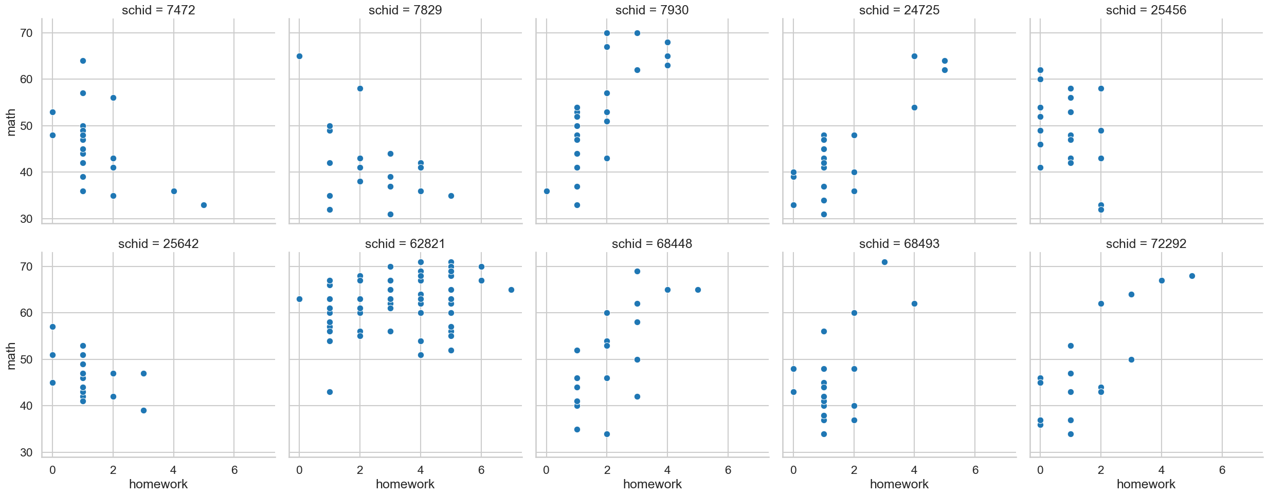
Can you use seaborn to visualise the association between homework and math for each of the ten schools, with a scatterplot?
Show code cell source
# Your answer here
# Visualise all associations
sns.relplot(data=school,
            x='homework', y='math',
            col='schid', col_wrap=5,
            kind='scatter')
<seaborn.axisgrid.FacetGrid at 0x128081e90>
Now, fit a simple GLM predicting math score from homework, which ignores the school id variable. We will use this to compare to a mixed model.
Show code cell source
# Your answer here
# GLM
glm = smf.ols('math ~ homework', data=school).fit()
glm.summary(slim=True)
| Dep. Variable: | math | R-squared: | 0.247 |
|---|---|---|---|
| Model: | OLS | Adj. R-squared: | 0.244 |
| No. Observations: | 260 | F-statistic: | 84.64 |
| Covariance Type: | nonrobust | Prob (F-statistic): | 1.25e-17 |
| coef | std err | t | P>|t| | [0.025 | 0.975] | |
|---|---|---|---|---|---|---|
| Intercept | 44.0739 | 0.989 | 44.580 | 0.000 | 42.127 | 46.021 |
| homework | 3.5719 | 0.388 | 9.200 | 0.000 | 2.807 | 4.336 |
Notes:
[1] Standard Errors assume that the covariance matrix of the errors is correctly specified.
Now, lets incorporate the variability from schools by giving a random intercept to schools, using a mixed model.
Show code cell source
# Your answer here
# Mixed models
mix = smf.mixedlm('math ~ homework',
                  groups='schid',
                  data=school).fit()
mix.summary()
| Model: | MixedLM | Dependent Variable: | math |
| No. Observations: | 260 | Method: | REML |
| No. Groups: | 10 | Scale: | 64.5228 |
| Min. group size: | 20 | Log-Likelihood: | -919.9738 |
| Max. group size: | 67 | Converged: | Yes |
| Mean group size: | 26.0 |
| Coef. | Std.Err. | z | P>|z| | [0.025 | 0.975] | |
|---|---|---|---|---|---|---|
| Intercept | 44.982 | 1.803 | 24.947 | 0.000 | 41.448 | 48.516 |
| homework | 2.207 | 0.381 | 5.798 | 0.000 | 1.461 | 2.952 |
| schid Var | 25.226 | 1.630 |
What happened to the association between homework and scores when incorporating the random effect of schools? Bonus points if you can plot the fitted values from the mixed model.
Next, let us add some more complexity. Our existing mixed model incorporates only each schools baseline maths score (a good way to find out which school is over-or-under-performing). It assumes the amount of homework completed has the same effect on maths exam scores for every school. That’ not realistic. Expand the model so it allows this effect to vary (e.g., a random slope for homework).
Show code cell source
# Your answer here
# mixed model with random slope
mix2 = smf.mixedlm('math ~ homework',
                   groups='schid',
                   re_formula='homework',
                   data=school).fit()

mix2.summary()
| Model: | MixedLM | Dependent Variable: | math |
| No. Observations: | 260 | Method: | REML |
| No. Groups: | 10 | Scale: | 43.0710 |
| Min. group size: | 20 | Log-Likelihood: | -881.9772 |
| Max. group size: | 67 | Converged: | Yes |
| Mean group size: | 26.0 |
| Coef. | Std.Err. | z | P>|z| | [0.025 | 0.975] | |
|---|---|---|---|---|---|---|
| Intercept | 44.771 | 2.744 | 16.314 | 0.000 | 39.392 | 50.149 |
| homework | 2.040 | 1.555 | 1.312 | 0.190 | -1.008 | 5.089 |
| schid Var | 69.304 | 5.437 | ||||
| schid x homework Cov | -31.762 | 2.812 | ||||
| homework Var | 22.453 | 1.787 |
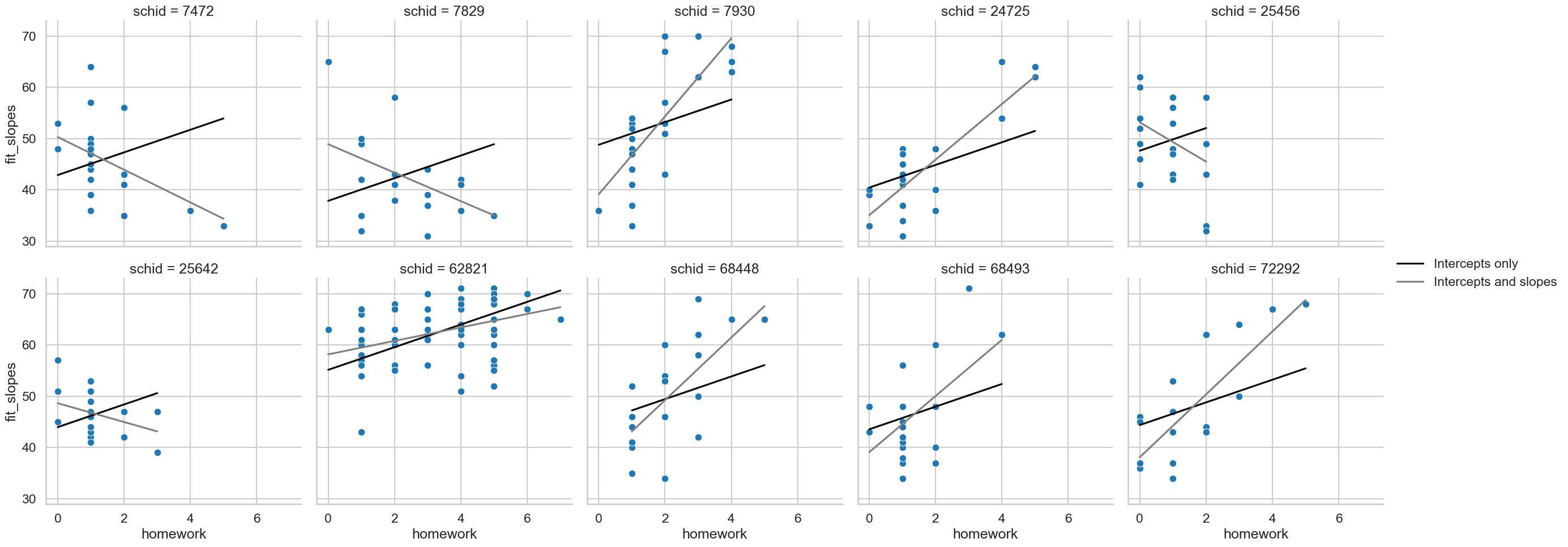
Now what happens to the association? More bonus points if you can include the predictions in a plot.
Show code cell source
# Your answer here
# Including fitted values
school['fit_slopes'] = mix2.fittedvalues
school['fit_intercept'] = mix.fittedvalues
(sns.relplot(data=school,
             x='homework', y='math',
             col='schid', col_wrap=5,
             kind='scatter')
 .map_dataframe(sns.lineplot, x='homework', y='fit_intercept', color='black', label='Intercepts only')
 .map_dataframe(sns.lineplot, x='homework', y='fit_slopes', color='grey', label='Intercepts and slopes')
 .add_legend()
)
<seaborn.axisgrid.FacetGrid at 0x1284b6610>
2. Cosmetics and attractiveness#
In the workshop we examined a model that included a random intercept for participants, a random intercept for models (both of those accounting for baseline levels of attractiveness ratings that each participant and model gives) and a random slope for cosmetics for each model (the model figures out the effect of a makeup application on the attractiveness of each model).
There’s at least one more effect that was not considered here, which is how makeup affects the perceptions of each rater. Each rater may differ in their response to cosmetics, with some liking it, and some being put off by it. Can you read in the data from the example and expand the model to include the random slope for raters too?
Show code cell source
# Your answer here
# Read in data
cosmetics = pd.read_csv('https://raw.githubusercontent.com/alexjonesphd/py4psy2024/refs/heads/main/jones_kramer_2015.csv')

# Add the grouping factor
cosmetics['grouping'] = 1

# Expand the random effects to include rater random slopes like this
re = {'pid': '0 + C(pid)',
      'model_id': '0 + C(model_id)',
      'cosmetics_model': '0 + C(model_id):cosmetics_code',
      'cosmetics_pid': '0 + C(pid):cosmetics_code'}

# Fit the odel
expand = smf.mixedlm('rating ~ cosmetics_code',
                     groups='grouping',
                     vc_formula=re,
                     data=cosmetics).fit()

expand.summary()
| Model: | MixedLM | Dependent Variable: | rating |
| No. Observations: | 3003 | Method: | REML |
| No. Groups: | 1 | Scale: | 1.4235 |
| Min. group size: | 3003 | Log-Likelihood: | -5048.0688 |
| Max. group size: | 3003 | Converged: | Yes |
| Mean group size: | 3003.0 |
| Coef. | Std.Err. | z | P>|z| | [0.025 | 0.975] | |
|---|---|---|---|---|---|---|
| Intercept | 3.231 | 0.152 | 21.265 | 0.000 | 2.933 | 3.529 |
| cosmetics_code | 1.163 | 0.145 | 8.008 | 0.000 | 0.878 | 1.448 |
| cosmetics_model Var | 0.514 | 0.122 | ||||
| cosmetics_pid Var | 0.322 | 0.063 | ||||
| model_id Var | 0.561 | 0.125 | ||||
| pid Var | 0.464 | 0.069 |
Once you have estimated this model, can you figure out what source of variation contributes the most to the attractiveness judgements out of:
Baseline attractiveness of models
Baseline tendency of attractiveness ratings of raters
Variation in the effect of cosmetics on models
Variation in the effect of cosmetics on participants?
Show code cell source
# Your answer here
# Sum up all random effects
total_variance = expand.vcomp.sum() + expand.scale

# Divide the vcomp by the total
expand.vcomp/total_variance
array([0.15664007, 0.09793443, 0.170859 , 0.14117325])
As an additional challenge - can you find the rater with the largest and smallest slope for cosmetics? This directly translates into someone for who cosmetics increased their ratings the most, and the one for who makeup was a major turn off. You will need to filter down the random effects which can be quite tricky.
Show code cell source
# Your answer here
# Convert random effects to a dataframe
ranef = pd.DataFrame(expand.random_effects)

# Filter it to include only PID and cosmetics_code
ppt_slopes = ranef[ranef.index.str.contains('cosmetics_code') & ranef.index.str.contains('pid')]

# With that, find the min + max
mini = ppt_slopes.idxmin()
maxi = ppt_slopes.idxmax()

print(mini, maxi)
1    cosmetics_pid[C(pid)[58]:cosmetics_code]
dtype: object 1    cosmetics_pid[C(pid)[75]:cosmetics_code]
dtype: object
3. Further challenges in linear mixed effects models#
Linear mixed models are, essentially, a standard GLM with extra flexibility to account for observations in the data belonging to groups. As such, they are able to incorporate all the usual things a GLM can. Here, we’ll use some more education data to examine whether there are differences between male and female A-level students on a Chemistry A-level score, and whether it is linked to their average GCSE score.
This data can be found from the Bristol Centre for Multilevel Modelling, here. Download the datasets, and upload the chem97.txt file to the server to access it. The code below will read in the file for you (assuming you have uploaded it) and rename the columns to something meaningful, but you can also see the readout on the above page for more detail.
Show code cell source
# Reads in data and renames columns
chem97 = pd.read_table('chem97.txt', sep='\s+', header=None)
chem97.columns = ['local_education_authority_ID', 'school_ID', 'pupil_ID', 'chem_Alevel_score', 'female', 'age_in_months', 'avg_GCSE']
chem97.head()
| local_education_authority_ID | school_ID | pupil_ID | chem_Alevel_score | female | age_in_months | avg_GCSE | |
|---|---|---|---|---|---|---|---|
| 0 | 1.0 | 1.0 | 1.0 | 4.0 | 1 | 3.0 | 6.625 |
| 1 | 1.0 | 1.0 | 2.0 | 10.0 | 1 | -3.0 | 7.625 |
| 2 | 1.0 | 1.0 | 3.0 | 10.0 | 1 | -4.0 | 7.250 |
| 3 | 1.0 | 1.0 | 4.0 | 10.0 | 1 | -2.0 | 7.500 |
| 4 | 1.0 | 1.0 | 5.0 | 8.0 | 1 | -1.0 | 6.444 |
Fit a linear mixed model that predicts chemistry A level score from the interaction between female (1 = yes, 0 = No) and aveage GCSE grade. Include random intercepts for education authority and school ID.
Show code cell source
# Your answer here
chem97['grouping'] = 1 # creates group

# create random effects
re = {'ed_authority': '0 + C(local_education_authority_ID)',
      'school': '0 + C(school_ID)'}

# Model - this MAY TAKE A WHILE!
md = smf.mixedlm('chem_Alevel_score ~ female * avg_GCSE',
                 groups='grouping',
                 vc_formula=re,
                 data=chem97).fit()

md.summary()
| Model: | MixedLM | Dependent Variable: | chem_Alevel_score |
| No. Observations: | 31022 | Method: | REML |
| No. Groups: | 1 | Scale: | 5.0495 |
| Min. group size: | 31022 | Log-Likelihood: | -70526.6060 |
| Max. group size: | 31022 | Converged: | Yes |
| Mean group size: | 31022.0 |
| Coef. | Std.Err. | z | P>|z| | [0.025 | 0.975] | |
|---|---|---|---|---|---|---|
| Intercept | -9.500 | 0.133 | -71.585 | 0.000 | -9.760 | -9.240 |
| female | -2.377 | 0.209 | -11.375 | 0.000 | -2.787 | -1.968 |
| avg_GCSE | 2.460 | 0.021 | 115.526 | 0.000 | 2.418 | 2.502 |
| female:avg_GCSE | 0.262 | 0.033 | 7.911 | 0.000 | 0.197 | 0.327 |
| ed_authority Var | 0.021 | 0.007 | ||||
| school Var | 1.125 | 0.025 |
With the model fitted, note the variance estimates and the coefficients. As with a GLM its not so easy to interpret whats going on - but we can rely on using average slopes to get conditional estimates, like always. Use marginaleffects to compute the slope for females and males with regards to GCSEs to explain the interaction.
Show code cell source
# Your answer here
# Get the slopes of GCSE for each sex
me.slopes(md, variables=['avg_GCSE'], by='female')
| female | term | contrast | estimate | std_error | statistic | p_value | s_value | conf_low | conf_high |
|---|---|---|---|---|---|---|---|---|---|
| i64 | str | str | f64 | f64 | f64 | f64 | f64 | f64 | f64 |
| 0 | "avg_GCSE" | "mean(dY/dX)" | 2.459902 | 0.021293 | 115.526716 | 0.0 | inf | 2.418169 | 2.501635 |
| 1 | "avg_GCSE" | "mean(dY/dX)" | 2.721689 | 0.02665 | 102.127443 | 0.0 | inf | 2.669456 | 2.773922 |
4. Studying individual differences with mixed models#
As a final example, lets see how mixed models can be used to understand measures of individual differences.
In the next dataset, we’ll see how individual raters are sensitive to facial cues of symmetry, averageness, and sexual dimorphism, three important predictors of facial attractiveness. Participants rated 100 faces on how attractive they thought they were (on a scale of 1-100). For each of the faces, we measured how symmetrical, distinctive, and sexually dimorphic it was.
First, read in the data from the following link and display the top 10 rows: https://raw.githubusercontent.com/alexjonesphd/py4psy2024/refs/heads/main/cue_sensitivity.csv
Show code cell source
# Your answer here
cues = pd.read_csv('https://raw.githubusercontent.com/alexjonesphd/py4psy2024/refs/heads/main/cue_sensitivity.csv')
cues.head(10)
| pid | face_id | face_sex | attractiveness | distinctiveness | symmetry | dimorphism | |
|---|---|---|---|---|---|---|---|
| 0 | 3168134.0 | galina | female | 44 | -1.535898 | -0.926857 | 0.056173 |
| 1 | 3168134.0 | tamara | female | 25 | 1.506863 | 0.567697 | -1.542840 |
| 2 | 3168134.0 | blazej | male | 50 | 1.066100 | -1.977071 | 0.758609 |
| 3 | 3168134.0 | irena | female | 58 | -1.196141 | -0.929967 | 0.751037 |
| 4 | 3168134.0 | jan | male | 27 | 0.039301 | 0.769465 | -0.082505 |
| 5 | 3168134.0 | svatopluk | male | 32 | -0.676461 | -1.102852 | -0.591465 |
| 6 | 3168134.0 | miroslav1 | male | 35 | 0.479499 | 1.627821 | -0.714593 |
| 7 | 3168134.0 | viola | female | 61 | -1.300203 | 1.283004 | 0.304360 |
| 8 | 3168134.0 | vincent | male | 2 | 0.715087 | -1.160949 | 1.252532 |
| 9 | 3168134.0 | blazana | female | 69 | -1.004162 | 0.838649 | -0.965687 |
Each participant rates 100 faces and we know the measurements of those faces. Lets fit a model that uses those measurements as predictors and accounts for participant and face variability with random slopes, as a starter.
Show code cell source
# Your answer here
cues['grouping'] = 1

# VC
vc = {'pid': '0 + C(pid)',
      'face': '0 + C(face_id)'}

# models
model1 = smf.mixedlm('attractiveness ~ distinctiveness + symmetry + dimorphism',
                     groups='grouping', vc_formula=vc, data=cues).fit()

model1.summary()
| Model: | MixedLM | Dependent Variable: | attractiveness |
| No. Observations: | 3200 | Method: | REML |
| No. Groups: | 1 | Scale: | 227.0840 |
| Min. group size: | 3200 | Log-Likelihood: | -13408.9376 |
| Max. group size: | 3200 | Converged: | Yes |
| Mean group size: | 3200.0 |
| Coef. | Std.Err. | z | P>|z| | [0.025 | 0.975] | |
|---|---|---|---|---|---|---|
| Intercept | 35.681 | 2.225 | 16.038 | 0.000 | 31.321 | 40.042 |
| distinctiveness | -2.398 | 1.013 | -2.367 | 0.018 | -4.383 | -0.413 |
| symmetry | -1.763 | 1.007 | -1.752 | 0.080 | -3.736 | 0.209 |
| dimorphism | -0.389 | 1.034 | -0.376 | 0.707 | -2.415 | 1.638 |
| face Var | 89.992 | 0.944 | ||||
| pid Var | 127.324 | 2.195 |
This model efffectively accounts for participant variability and face variability, and suggests only distinctiveness decreases attractiveness. But we must be clear on what it implies - it says that the effect of, say, distinctiveness is exactly the same for all raters. That is, raters are influenced by the distinctiveness of the face in the same way. Is this realistic? Would it be better to allow each rater their own distinctiveness slope (as well as others) to allow their own preferences to come out? We can do this of course by including a random slope for each rater for each trait. Do that below and see what happens.
Show code cell source
# Your answer here
# VC
re = {'pid': '0 + C(pid)',
      'face': '0 + C(face_id)',
      'distinctiveness': '0 + C(pid):distinctiveness',
      'symmetry': '0 + C(pid):symmetry',
      'dimorphism': '0 + C(pid):dimorphism'}

# models
model2 = smf.mixedlm('attractiveness ~ distinctiveness + symmetry + dimorphism',
                     groups='grouping', vc_formula=re, data=cues).fit()

model2.summary()
/opt/miniconda3/envs/py11/lib/python3.11/site-packages/statsmodels/base/model.py:607: ConvergenceWarning: Maximum Likelihood optimization failed to converge. Check mle_retvals
/opt/miniconda3/envs/py11/lib/python3.11/site-packages/statsmodels/regression/mixed_linear_model.py:2201: ConvergenceWarning: Retrying MixedLM optimization with lbfgs
/opt/miniconda3/envs/py11/lib/python3.11/site-packages/statsmodels/regression/mixed_linear_model.py:2262: ConvergenceWarning: The Hessian matrix at the estimated parameter values is not positive definite.
| Model: | MixedLM | Dependent Variable: | attractiveness |
| No. Observations: | 3200 | Method: | REML |
| No. Groups: | 1 | Scale: | 222.5967 |
| Min. group size: | 3200 | Log-Likelihood: | -13424.8905 |
| Max. group size: | 3200 | Converged: | Yes |
| Mean group size: | 3200.0 |
| Coef. | Std.Err. | z | P>|z| | [0.025 | 0.975] | |
|---|---|---|---|---|---|---|
| Intercept | 35.681 | 2.282 | 15.633 | 0.000 | 31.208 | 40.155 |
| distinctiveness | -2.398 | 1.517 | -1.581 | 0.114 | -5.371 | 0.575 |
| symmetry | -1.763 | 1.509 | -1.169 | 0.243 | -4.721 | 1.194 |
| dimorphism | -0.389 | 1.549 | -0.251 | 0.802 | -3.425 | 2.648 |
| dimorphism Var | 0.670 | 0.121 | ||||
| distinctiveness Var | 0.591 | 0.060 | ||||
| face Var | 209.005 | |||||
| pid Var | 97.593 | 1.352 | ||||
| symmetry Var | 0.769 | 0.143 |
Now the effects go away when you consider how variable these effects are for people. If we wanted, we could extract each persons individual slope to see how sensitive they are to an individual cue.