6 - Precision in Predictions

Figuring out precision and other types of tests

There are only a few examples this week to drive home the idea of precision in predictions, or equivalently, how uncertain we are of our predictions.

The main take home message is that our predictions will vary in precision, but that the impact of this precision varies with the magnitude of the effect. A large prediction that is imprecise may be of more use than a tiny, precise prediction - as ever, it all depends on the use of the model. Traditionally, p-values will be significant when precision is high, with comes with larger sample sizes. We must not be misled by significance, and should think carefully about what kind of hypotheses are important about our predictions.

Finding precision

We will see some examples of precision in prediction. First, lets import all the usual packages we need:

# Import what we need
import pandas as pd # dataframes
import seaborn as sns # plots
import statsmodels.formula.api as smf # Models
import marginaleffects as me # marginal effects
import numpy as np # numpy for some functions

# Set the style for plots
sns.set_style('whitegrid')
sns.set_context('talk')

Intervention data

We will load the data for the childhood intervention study to examine prediction and precision in some detail, and explore how to set specific hypotheses to test.

We download it from here: https://vincentarelbundock.github.io/Rdatasets/csv/mlmRev/Early.csv

# Read in 
cog = pd.read_csv('https://vincentarelbundock.github.io/Rdatasets/csv/mlmRev/Early.csv')
cog.head()

	rownames	id	cog	age	trt
0	1	68	103	1.0	Y
1	2	68	119	1.5	Y
2	3	68	96	2.0	Y
3	4	70	106	1.0	Y
4	5	70	107	1.5	Y

And fit a simple model to the data:

# Model
cog_mod = smf.ols('cog ~ age + trt', data=cog).fit()
cog_mod.summary(slim=True)

OLS Regression Results

Dep. Variable:	cog	R-squared:	0.314
Model:	OLS	Adj. R-squared:	0.309
No. Observations:	309	F-statistic:	69.97
Covariance Type:	nonrobust	Prob (F-statistic):	9.45e-26

	coef	std err	t	P>|t|	[0.025	0.975]
Intercept	124.5216	2.950	42.206	0.000	118.716	130.327
trt[T.Y]	9.4903	1.497	6.340	0.000	6.545	12.436
age	-18.1650	1.819	-9.988	0.000	-21.744	-14.586

Notes:
[1] Standard Errors assume that the covariance matrix of the errors is correctly specified.

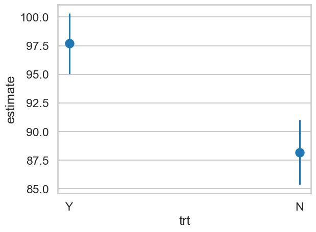
We can then predict the effect of the intervention for 2 year olds easily:

# Predict for 2 year olds
p = me.predictions(cog_mod,
                   newdata=me.datagrid(cog_mod,
                                       trt=['Y', 'N'],
                                       age=2)
                  )

p

shape: (2, 13)

trt	age	rowid	estimate	std_error	statistic	p_value	s_value	conf_low	conf_high	rownames	id	cog
str	i64	i32	f64	f64	f64	f64	f64	f64	f64	i64	i64	i64
"Y"	2	0	97.681844	1.343884	72.68623	0.0	inf	95.04788	100.315807	89	966	96
"N"	2	1	88.19155	1.445289	61.019992	0.0	inf	85.358835	91.024265	89	966	96

The conf_low and conf_high represent the 95% confidence interval bounds.

# Plot
ax = sns.pointplot(data=p,
                   x='trt', y='estimate',
                   linestyle='none')
# Add errors
ax.vlines(p['trt'], p['conf_low'], p['conf_high'])

<matplotlib.collections.LineCollection at 0x177ec3c90>

Testing hypotheses

We can compute the difference between these two as usual with the hypothesis argument, and obtain the interval around the difference:

# Difference
p = me.predictions(cog_mod,
                   newdata=me.datagrid(cog_mod,
                                       trt=['Y', 'N'],
                                       age=2),
                   hypothesis='b1=b2')
p

shape: (1, 8)

term	estimate	std_error	statistic	p_value	s_value	conf_low	conf_high
str	f64	f64	f64	f64	f64	f64	f64
"b1=b2"	9.490294	1.49698	6.339628	2.3032e-10	32.015641	6.556268	12.42432

# Plot
ax = sns.pointplot(data=p,
                   x='term', y='estimate',
                   linestyle='none')
# Add errors
ax.vlines(p['term'], p['conf_low'], p['conf_high'])

<matplotlib.collections.LineCollection at 0x177f25f50>

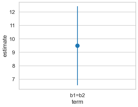
The p-value of this difference is significant, as it shows that we’d not expect to see a difference as large as this if the difference between the interventions was zero.

But that’s often a bit of a silly hypothesis to begin with. We’d not run the intervention (or study, or wherever we get our data!) if we thought the difference was really nothing to start with.

Instead, imagine the scenario that your new intervention is out to beat an existing one. That one showed a difference of 7 units by age 2. Is this intervention better than that? Testing this is simple:

# Difference
p = me.predictions(cog_mod,
                   newdata=me.datagrid(cog_mod,
                                       trt=['Y', 'N'],
                                       age=2),
                   hypothesis='b1-b2 = 7') 
# Subtract one from the other, is it equal to 7?
p

shape: (1, 8)

term	estimate	std_error	statistic	p_value	s_value	conf_low	conf_high
str	f64	f64	f64	f64	f64	f64	f64
"b1-b2=7"	2.490294	1.49698	1.663546	0.096203	3.37777	-0.443732	5.42432

The predicted difference from seven - not zero - is about 2.5, and it is not significant. But note the confidence interval - it might be just less than 7, or quite a bit above it. So while it is not statistically significant, this might well be worth pursuing! This is an example of a large prediction with a wide interval. If the null value is zero this is comfortably significant, but if its 7, it is not - but the interval indicates the effect could be rather a bit larger than 7. Circumstance dictates what the appropriate outcome is.

You can test almost any hypothesis with marginaleffects with a careful application, and often, the hypothesis of zero is not that interesting!

Testing an interval hypothesis

We can also express a hypothesis as an interval.

Imagine this somewhat complex scenario:

• A previous, more expensive intervention produces a change of 7 points.

• We are tasked with seeing if our intervention is at least as good as - i.e., is equivalent to the existing one, for children aged 2.

• The current intervention will replace the existing one, if it can be shown to be equivalent to give an increase of at least 6.5 - 12.5.

• The developers would like it to be better than 7, but they’ll accept anywhere between 6.5 and 12.5 as equivalent.

Testing this kind of ‘interval’ hypothesis is easy, but a bit confusing philosophically. A significant result means our estimate is within the bounds specified, a non-significant one indicating one or both of the bounds are within the confidence interval and cannot be excluded - i.e., the effect could be lower than 6.5 or bigger than 12.5. We do this using the equivalence keyword and a list of the lower and upper bounds, in addition to the standard hypothesis:

# Equivalence
eq = me.predictions(cog_mod,
                    newdata=me.datagrid(cog_mod,
                                        trt=['Y', 'N'],
                                        age=2),
                    hypothesis='b1=b2',
                    equivalence=[6.5, 12.5])
eq

shape: (1, 13)

term	estimate	std_error	statistic	p_value	s_value	conf_low	conf_high	statistic_noninf	statistic_nonsup	p_value_noninf	p_value_nonsup	p_value_equiv
str	f64	f64	f64	f64	f64	f64	f64	f64	f64	f64	f64	f64
"b1=b2"	9.490294	1.49698	6.339628	2.3032e-10	32.015641	6.556268	12.42432	1.997552	-2.010519	0.022883	0.022188	0.022883

The p_value_equiv contains the information we need. Illustrating this graphically:

# Plot
ax = sns.pointplot(data=eq, x='term', y='estimate')
ax.vlines(eq['term'], eq['conf_low'], eq['conf_high'])
ax.axhline(6.5)
ax.axhline(12.5)

<matplotlib.lines.Line2D at 0x16aa8b990>

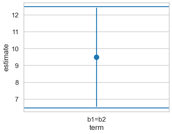
This technique can be very useful. Sometimes you may see a small, precise, and significant result. Rather than taking this as evidence, we may test whether the result is within an interval of effects we could consider either important or unimportant (the definition is up to you!), and test that.

The downside is that defining these intervals is difficult, requires justification, and can be frowned on by less statistically literate folk.

One more example

Lets consider another example, revisiting the beauty and wages dataset. First, we read it in and fit a simple model where we predict hourly wages from a looks variable that goes from 1 to 5, and an exper variable that counts the persons years of experience in the workforce. This shows a statistically significant effect of looks and experience:

# Read in looks
looks = pd.read_csv('https://vincentarelbundock.github.io/Rdatasets/csv/wooldridge/beauty.csv')

# Fit a simple model and examine output
looks_mod = smf.ols('wage ~ exper + looks', data=looks).fit()
looks_mod.summary(slim=True)

OLS Regression Results

Dep. Variable:	wage	R-squared:	0.064
Model:	OLS	Adj. R-squared:	0.062
No. Observations:	1260	F-statistic:	42.70
Covariance Type:	nonrobust	Prob (F-statistic):	1.15e-18

	coef	std err	t	P>|t|	[0.025	0.975]
Intercept	2.5094	0.671	3.742	0.000	1.194	3.825
exper	0.0971	0.011	9.018	0.000	0.076	0.118
looks	0.6373	0.188	3.390	0.001	0.268	1.006

Notes:
[1] Standard Errors assume that the covariance matrix of the errors is correctly specified.

As a silly example, lets assume taking up regular exercise, clean eating, and expensive beauty products will shift your looks from a 3 to a 4. Averaging over your years of experience, how much does going from a 3 to a 4 increase your hourly wage?

# Make a datagrid
dg = me.datagrid(looks_mod,
                 looks=[3, 4],
                 exper=np.arange(1, 40)
                )

# Make the predictions
p = me.predictions(looks_mod,
                   newdata=dg,
                   by='looks') # average over experience

p

shape: (2, 8)

looks	estimate	std_error	statistic	p_value	s_value	conf_low	conf_high
i64	f64	f64	f64	f64	f64	f64	f64
3	6.362436	0.132481	48.025307	0.0	inf	6.102778	6.622094
4	6.999705	0.202224	34.61356	0.0	inf	6.603352	7.396057

With looks of about 3, you earn 6.36 an hour. With a four, you earn basically 7. Is this difference statistically significant?

# Include hypothesis of zero difference, test to reject
me.predictions(looks_mod,
               newdata=dg,
               by='looks',
               hypothesis='b2 - b1 = 0') # Same as b2=b1 or 4 - 3

shape: (1, 8)

term	estimate	std_error	statistic	p_value	s_value	conf_low	conf_high
str	f64	f64	f64	f64	f64	f64	f64
"b2-b1=0"	0.637269	0.188008	3.389585	0.0007	10.480386	0.26878	1.005757

The difference of about 0.64 is significant. Hold on though, all that exercise, expensive products and good food is a LOT of effort. Will it earn you at least an extra 0.50 an hour?

# Include hypothesis of a 50-cent difference, test to reject
me.predictions(looks_mod,
               newdata=dg,
               by='looks',
               hypothesis='b2 - b1 = 0.50') 

shape: (1, 8)

term	estimate	std_error	statistic	p_value	s_value	conf_low	conf_high
str	f64	f64	f64	f64	f64	f64	f64
"b2-b1=0.50"	0.137269	0.188008	0.730122	0.465316	1.103719	-0.23122	0.505757

This difference is not statistically significant, so you conclude the conclude there’s no evidence it will improve your wages above 50 cents an hour.

Imagine now you say - this increase of a 3 to a 4 is going to be a lot of work.

Anything from an increase of 0.01 to 1 dollar is absolutely not worth it, and so I’ll consider that increase equivalent to what I currently earn - all the gym memberships and beauty products will cost me more than that. An increase of 0.01 to 1 dollar is my interval hypothesis.

You can test that hypothesis like so:

# Equivalence hypothesis
eq = me.predictions(looks_mod,
                    newdata=dg,
                    by='looks',
                    hypothesis='b2 - b1 = 0',
                    equivalence=[0.01, 1.])
eq

shape: (1, 13)

term	estimate	std_error	statistic	p_value	s_value	conf_low	conf_high	statistic_noninf	statistic_nonsup	p_value_noninf	p_value_nonsup	p_value_equiv
str	f64	f64	f64	f64	f64	f64	f64	f64	f64	f64	f64	f64
"b2-b1=0"	0.637269	0.188008	3.389585	0.0007	10.480386	0.26878	1.005757	3.336395	-1.929341	0.000424	0.026844	0.026844

This is significant, which indicates the effect is within the interval, and thus you can conclude the end result is the same as what you presently earn:

# Plot
ax = sns.pointplot(data=eq, x='term', y='estimate')
ax.vlines(eq['term'], eq['conf_low'], eq['conf_high'])
ax.axhline(0.01)
ax.axhline(1)

<matplotlib.lines.Line2D at 0x30c3f7b50>

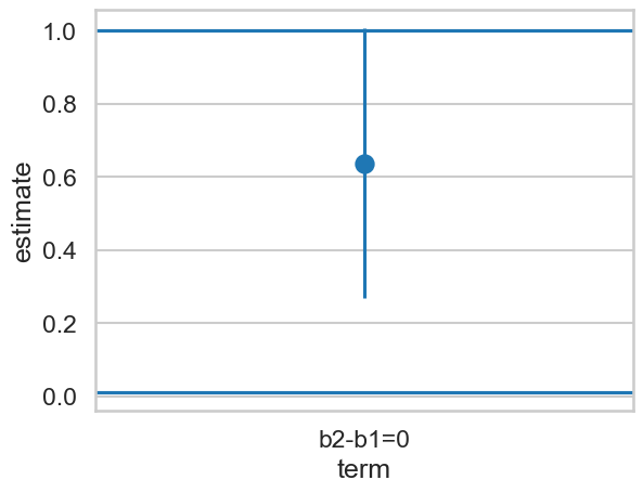
To reiterate, this test is significant, which means you can say the effect is unintersting, null, or too small to be of interest. If the test was not significant, you would conclude that the intervention on your looks could possibly yield effects outside of this interval and thus could be of interest.