5 - Binary outcome models

Dealing with non-continuous outcomes

This week we expand our linear model knowledge to deal with binary outcomes. That is - sticking to the mantra of ‘all models are wrong, but some are useful’, how can we best model and understand data that only ever takes on one of two values?

Probit regression

Probit regression solves this problem. Many of the same skills used for the GLM apply here, so we will spend some time fitting probit models using statsmodels, examining their probabilistic predictions with marginaleffects, and calculating some of thei varied statistics with other tools.

Lets import everything we need for now:

# Import most of what we need
import pandas as pd # dataframes
import seaborn as sns # plots
import statsmodels.formula.api as smf # Models
import marginaleffects as me # marginal effects

# Set the style for plots
sns.set_style('ticks') # a different theme!
sns.set_context('talk')

Dichotomising data

We will continue the example of working with the affairs dataset, but this time focusing on a binary outcome. First, we will load the dataset, and observe that the affair column has multiple distinct values:

# First read in the data
affairs = pd.read_csv('https://vincentarelbundock.github.io/Rdatasets/csv/AER/Affairs.csv')

# Show top 3
display(affairs.head(3))

# Show the unique values in the affair columns
print(affairs['affairs'].value_counts())

	rownames	affairs	gender	age	yearsmarried	children	religiousness	education	occupation	rating
0	4	0	male	37.0	10.0	no	3	18	7	4
1	5	0	female	27.0	4.0	no	4	14	6	4
2	11	0	female	32.0	15.0	yes	1	12	1	4

affairs
0     451
7      42
12     38
1      34
3      19
2      17
Name: count, dtype: int64

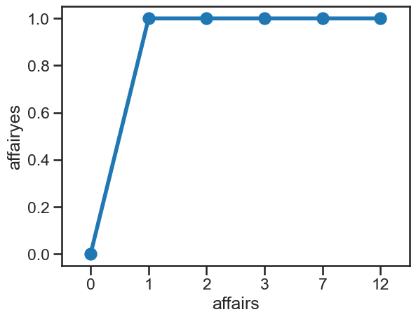
This suggests the majoirty of people have not had an affair, while a minority have had one or more. To use a probit regression here - to predict whether someone has, or has not, then we need to dichotomise the variable and put it back into the dataframe.

A quick way of doing this is to borrow a function from a package called numpy, called digitize. This takes a column of a dataframe and a list of thresholds, and recodes the data such that equal to the threshold or more gets replaced with that value.

Lets import numpy and recode the affairs column.

# Import numpy with alias
import numpy as np

# Digitise the affairs column for 1 or more, put into a new column in the dataframe
affairs['affairyes'] = np.digitize(affairs['affairs'], [1])

# Scatter
sns.pointplot(data=affairs, x='affairs', y='affairyes')

<Axes: xlabel='affairs', ylabel='affairyes'>

Fitting a model and making predictions

With the new dichomotised variable, fitting a model is as simple as using statsmodels to use probit instead of ols.

Below we predict occurrence of an affair from marriage rating, children, and years of marriage.

# Fitting a probit model
probit_model = smf.probit('affairyes ~ rating + yearsmarried + children',
                          data=affairs).fit()

# Show summary
probit_model.summary()

Optimization terminated successfully.
         Current function value: 0.525523
         Iterations 5

Probit Regression Results

Dep. Variable:	affairyes	No. Observations:	601
Model:	Probit	Df Residuals:	597
Method:	MLE	Df Model:	3
Date:	Fri, 01 Nov 2024	Pseudo R-squ.:	0.06470
Time:	00:54:58	Log-Likelihood:	-315.84
converged:	True	LL-Null:	-337.69
Covariance Type:	nonrobust	LLR p-value:	1.749e-09

	coef	std err	z	P>|z|	[0.025	0.975]
Intercept	0.0852	0.252	0.338	0.735	-0.409	0.579
children[T.yes]	0.2243	0.160	1.404	0.160	-0.089	0.538
rating	-0.2739	0.052	-5.299	0.000	-0.375	-0.173
yearsmarried	0.0136	0.012	1.088	0.277	-0.011	0.038

We can roughly interpret this outcome along the lines of those who are happier in their marriage move lower down the unobserved ‘tendency to engage in an affair’ variable, i.e., it reduces their probability of an affair. But by how much requires examining predictions - reasoning about coefficients in the GLM is hard, but with probit models it is even harder.

Luckily, marginaleffects works exactly the same way. Lets have the model predict the probabilities of an affair for individuals with each level of marital satisfaction, just like with the GLM:

# Predictions
predict_for = me.datagrid(probit_model,
                          rating=[1, 2, 3, 4, 5])

# Predictions
predictions = me.predictions(probit_model, 
                             newdata=predict_for)

# Display
display(predictions)

shape: (5, 19)

rating	rowid	estimate	std_error	statistic	p_value	s_value	conf_low	conf_high	rownames	affairs	gender	age	yearsmarried	children	religiousness	education	occupation	affairyes
i64	i32	f64	f64	f64	f64	f64	f64	f64	i64	i64	str	f64	f64	str	i64	i64	i64	i64
1	0	0.55826	0.062539	8.926567	0.0	inf	0.435685	0.680834	217	0	"female"	32.487521	8.177696	"yes"	4	14	5	0
2	1	0.449339	0.045342	9.910018	0.0	inf	0.360471	0.538208	217	0	"female"	32.487521	8.177696	"yes"	4	14	5	0
3	2	0.344129	0.029661	11.602137	0.0	inf	0.285995	0.402263	217	0	"female"	32.487521	8.177696	"yes"	4	14	5	0
4	3	0.249803	0.022909	10.904162	0.0	inf	0.204902	0.294703	217	0	"female"	32.487521	8.177696	"yes"	4	14	5	0
5	4	0.17131	0.024463	7.002925	2.5067e-12	38.53737	0.123364	0.219256	217	0	"female"	32.487521	8.177696	"yes"	4	14	5	0

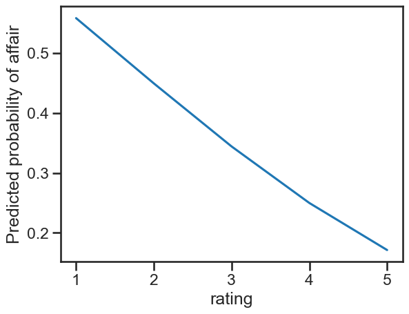
If we plot this we see the slightly non-linear relationship:

# Plot
ax = sns.lineplot(data=predictions,
                  x='rating', y='estimate')
ax.set(ylabel='Predicted probability of affair')

[Text(0, 0.5, 'Predicted probability of affair')]

The predictions work in the same fashion as the GLM. For example, we can ask whether those with the highest satisfaction of 5 are less likely to have an affair than those with a 4:

# Contrast a 4 and 5
me.predictions(probit_model, 
               newdata=me.datagrid(rating=[5, 4]),
               hypothesis='pairwise')

shape: (1, 8)

term	estimate	std_error	statistic	p_value	s_value	conf_low	conf_high
str	f64	f64	f64	f64	f64	f64	f64
"Row 1 - Row 2"	-0.078493	0.013093	-5.995016	2.0347e-9	28.872566	-0.104154	-0.052831

Those with a satisfaction of 5 have a lower probability of engaging in an affair of about 8 points, which is statistically significant. Notice how this number is totally divorced from the coefficients - in a GLM there would be some correspondence, but here, the predictions are absolutely essential.

As a further example, consider the difference between those with a 1 and 2 on the satisfaction scale:

# Contrast a 1 and 2
me.predictions(probit_model, 
               newdata=me.datagrid(rating=[2, 1]),
               hypothesis='pairwise')

shape: (1, 8)

term	estimate	std_error	statistic	p_value	s_value	conf_low	conf_high
str	f64	f64	f64	f64	f64	f64	f64
"Row 1 - Row 2"	-0.108921	0.020308	-5.363511	8.1620e-8	23.546511	-0.148723	-0.069118

This is around 11 points - this is not the same as the 5 - 4 difference, which it would be in a GLM, because they are absolutely linear, while these models are not! The distinction is subtle but vital in interpretation, but since we are used to dealing with predictions, we need not worry.

Checking fit and other statistics

Lets see how to examine a range of statistics related to the fit of a probit model.

The log-likelihood statistic

First, the log-likelihood statistic, which shows us whether the predictors improve the predictions over a model with no predictors. This is stored in the .summary() output - a value closer to zero is better:

# Show summary, just first table
probit_model.summary().tables[0]

Probit Regression Results

Dep. Variable:	affairyes	No. Observations:	601
Model:	Probit	Df Residuals:	597
Method:	MLE	Df Model:	3
Date:	Fri, 01 Nov 2024	Pseudo R-squ.:	0.06470
Time:	00:54:58	Log-Likelihood:	-315.84
converged:	True	LL-Null:	-337.69
Covariance Type:	nonrobust	LLR p-value:	1.749e-09

This is significant, offering us a coarse measure that our predictors, at least, aren’t making things worse!

The phi coefficient

This is the correlation between the observed values and predicted binary values. This takes a little bit of work to obtain, with the following steps:

• Obtain the predicted probabilities of each datapoint

• Convert them to 0 and 1 depending on whether they are below or above .5

• Correlate them with the observed data, using the corr function from pingouin.

We can do this in a few steps, relying on marginaleffects and the handy np.digitize function.

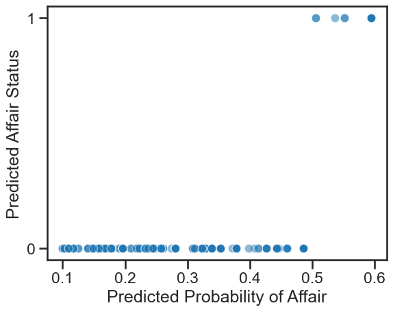
First, get the predictions for each data point, then dichotomise them.

# First make a prediction on the whole dataset, like so
all_predictions = me.predictions(probit_model) 
# notice there's nothing else here bar the model

# Digitize with .5 as the threshold
binary_predictions = np.digitize(all_predictions['estimate'],
                                 [0.5])

# Plot
ax = sns.scatterplot(x=all_predictions['estimate'],
                     y=binary_predictions,
                     alpha=.5)
ax.set(yticks=[0, 1],
       ylabel='Predicted Affair Status',
       xlabel='Predicted Probability of Affair')
       

[[<matplotlib.axis.YTick at 0x151e99e90>,
  <matplotlib.axis.YTick at 0x151ead8d0>],
 Text(0, 0.5, 'Predicted Affair Status'),
 Text(0.5, 0, 'Predicted Probability of Affair')]

Next, we import pingouin and carry out the correlation between the observed and actual values.

# Import pingouin
import pingouin as pg

# Correlate
pg.corr(affairs['affairyes'],
        binary_predictions)

	n	r	CI95%	p-val	BF10	power
pearson	601	0.080253	[0.0, 0.16]	0.04924	0.352	0.503309

Note the barely significant correlation here. The phi coefficient is not too promising, despite the other statistics!

The confusion matrix

Now we have the binary predictions in hand, we can build the confusion matrix that lets us interpret the types of predictions the model has made. We can rely on pandas to help us figure this out, using the pd.crosstab function, which will neatly tabulate our results. All it needs is the actual data, and the predicted data, like so:

# Crosstabs
pd.crosstab(affairs['affairyes'],
            binary_predictions,
            rownames=['Observed'], # labels the rows
            colnames=['Predicted'], # labels the columns
            margins=True) # calculates the totals across rows and columns

Predicted	0	1	All
Observed
0	443	8	451
1	143	7	150
All	586	15	601

We can now see the explanation for the low phi coefficient. The model is making a lot of false negative predictions. That is, it is labelling those who have had an affair (150 in the data) as not having done so - out of the 150 who have, it thinks 143 did not, and only gets 7 correct!

So as to dispel confusion about confusion matrices, here are the kinds of predictions this model has made:

• True negatives - The model correctly predicted 0 for 443 people who did not have an affair, out of 451 who did not.

• True positives - the model correctly predicted 1 for 7 people who did have an affair, out of 150 who did.

• False negatives - the model incorrectly predicted 0 for 143 who did have an affair, out of the 150 who did.

• False positives - the model incorrectly predicted 1 for 8 people who did not have an affair, out of the 451 who did.

For a model designed to predict those who might engage in an affair, this is not great!

Building complexity in a probit model

Having evaluated the model and found it lacking, lets try to improve it. One clear way is to increase the complexity by adding in interactions.

Here we test a model that has a more complex story. We adjust for marital satisfaction ratings, but we include an interaction between years married, child status, and gender. This supposes that the propensity of an affair alters for how long a couple has been married and their child status, and that this pattern may be different for males and females.

# Fitting a probit model
probit_model2 = smf.probit('affairyes ~ rating + yearsmarried * children * gender',
                          data=affairs).fit()

# Show summary
probit_model2.summary()

Optimization terminated successfully.
         Current function value: 0.518543
         Iterations 6

Probit Regression Results

Dep. Variable:	affairyes	No. Observations:	601
Model:	Probit	Df Residuals:	592
Method:	MLE	Df Model:	8
Date:	Fri, 01 Nov 2024	Pseudo R-squ.:	0.07713
Time:	00:54:58	Log-Likelihood:	-311.64
converged:	True	LL-Null:	-337.69
Covariance Type:	nonrobust	LLR p-value:	1.618e-08

	coef	std err	z	P>|z|	[0.025	0.975]
Intercept	-0.4448	0.340	-1.308	0.191	-1.111	0.222
children[T.yes]	0.8571	0.340	2.522	0.012	0.191	1.523
gender[T.male]	0.5388	0.350	1.541	0.123	-0.147	1.224
children[T.yes]:gender[T.male]	-0.5331	0.464	-1.148	0.251	-1.443	0.377
rating	-0.2698	0.052	-5.158	0.000	-0.372	-0.167
yearsmarried	0.1327	0.052	2.540	0.011	0.030	0.235
yearsmarried:children[T.yes]	-0.1350	0.056	-2.421	0.015	-0.244	-0.026
yearsmarried:gender[T.male]	-0.0922	0.065	-1.412	0.158	-0.220	0.036
yearsmarried:children[T.yes]:gender[T.male]	0.1008	0.071	1.429	0.153	-0.037	0.239

A few coefficients, including part of the interaction, are significant, and the log-likelihood ratio test is also.

Let’s make sense of this interaction step-by-step. First, we will generate and plot the predictions for a range of candidate years of marriage, for those with and without children, and for females and males:

# Plot predictions
predict_this = me.datagrid(probit_model2,
                           yearsmarried=np.arange(1, 25), # generates numbers 1 to 25
                           children=['yes', 'no'],
                           gender=['male', 'female'])

# Get probabilities!
probs = me.predictions(probit_model2, 
                       newdata=predict_this)

# Plot
g = sns.relplot(data=probs,
                x='yearsmarried', y='estimate',
                hue='children', col='gender',
                kind='line', palette='magma')
g.refline(y=0.5)
g.set_ylabels('Predicted Probability of an Affair')
g.set_xlabels('Years Married')
g.set(xticks=[1, 5, 10, 15, 20, 25])

<seaborn.axisgrid.FacetGrid at 0x151e579d0>

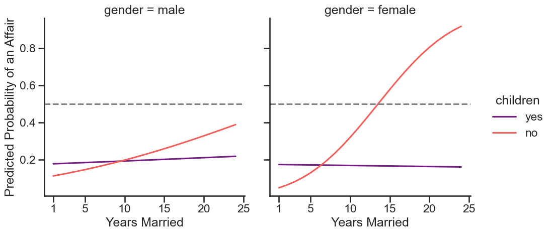
This suggests that while males and females with children have more or less a constant probability of an affair across their marriage duration, there is an increase in probabilities for those without children, and particularly for females.

We can explore this further by examining the slopes of years married for females and males, with and without children:

# Slopes
me.slopes(probit_model2,
          newdata=predict_this,
          variables='yearsmarried',
          by=['gender', 'children'])

shape: (4, 11)

children	gender	term	contrast	estimate	std_error	statistic	p_value	s_value	conf_low	conf_high
str	str	str	str	f64	f64	f64	f64	f64	f64	f64
"no"	"female"	"yearsmarried"	"mean(dY/dX)"	0.0369	0.006906	5.343087	9.1377e-8	23.383592	0.023364	0.050436
"yes"	"female"	"yearsmarried"	"mean(dY/dX)"	-0.000573	0.004898	-0.11705	0.90682	0.141111	-0.010172	0.009026
"no"	"male"	"yearsmarried"	"mean(dY/dX)"	0.011999	0.013958	0.859613	0.390002	1.358445	-0.015359	0.039356
"yes"	"male"	"yearsmarried"	"mean(dY/dX)"	0.001757	0.005161	0.340349	0.733593	0.446947	-0.00836	0.011873

These demonstrate the slope (at its maximum point) for each combination of male, female, and child status.

We can then test the hypotheses about whether these slopes are different using hypothesis methods. Is there a higher slope for females without children than with?

# First hypothesis
me.slopes(probit_model2,
          newdata=predict_this,
          variables='yearsmarried',
          by=['gender', 'children'],
          hypothesis='b1=b2')

shape: (1, 8)

term	estimate	std_error	statistic	p_value	s_value	conf_low	conf_high
str	f64	f64	f64	f64	f64	f64	f64
"b1=b2"	0.037474	0.008454	4.432489	0.000009	16.711988	0.020903	0.054044

And for males:

# Second hypothesis
me.slopes(probit_model2,
          newdata=predict_this,
          variables='yearsmarried',
          by=['gender', 'children'],
          hypothesis='b3=b4')

shape: (1, 8)

term	estimate	std_error	statistic	p_value	s_value	conf_low	conf_high
str	f64	f64	f64	f64	f64	f64	f64
"b3=b4"	0.010242	0.014848	0.689767	0.49034	1.028144	-0.01886	0.039344

So an effect for females, not for males. Is the difference in these differences significant?

# Compound hypothesis
me.slopes(probit_model2,
          newdata=predict_this,
          variables='yearsmarried',
          by=['gender', 'children'],
          hypothesis='b1-b2 = b3-b4') # Females No - Yes = Male No - Yes

shape: (1, 8)

term	estimate	std_error	statistic	p_value	s_value	conf_low	conf_high
str	f64	f64	f64	f64	f64	f64	f64
"b1-b2=b3-b4"	0.027232	0.017103	1.592185	0.111343	3.166916	-0.00629	0.060754

Almost; but not quite. But as we’ve seen, significance is not everything - we must also examine whether the model is doing a good job at predicting the data in terms of its classifications. First, we can compute the phi coefficient:

# Phi coeff
# Predictions for all data
all_predictions = me.predictions(probit_model2) 

# Digitize with .5 as the threshold
binary_predictions = np.digitize(all_predictions['estimate'],
                                 [0.5])

# Correlate
pg.corr(affairs['affairyes'], binary_predictions)

	n	r	CI95%	p-val	BF10	power
pearson	601	0.101673	[0.02, 0.18]	0.012638	1.136	0.704305

And the final check is to look at the confusion matrix:

# Confusion matrix
pd.crosstab(affairs['affairyes'],
            binary_predictions,
            rownames=['Observed'],
            colnames=['Predicted'])

Predicted	0	1
Observed
0	442	9
1	141	9

With these two extra pieces of information, its clear the model is not particularly good. Caution and circumspection is always warranted.