1 - Introduction#
Using Python for Data Analysis#
Python is a vast programming language with almost unlimited flexibility. Our focus in this module will be to use it to:
Read data and do basic manipulations of it
Fit statistical models to this data
Visualise the data through plots
While there are a range of uses for the tools we will cover, particularly the art of ‘data wrangling’, these are outside the scope of the content. You will however get the skills to learn these more advanced approaches and there are many resources to advance you.
Part 1 - Basic syntax#
Here, we take a look at the basic syntax, or rules, we can use to get Python working for us.
# This is a comment.
# Anything following the '#' symbol is ignored, but it lets us write notes to ourselves
Python is capable of very basic mathematical operations!
# Addition
print(10 + 5)

# Subtraction
print(10 - 5)

# Division
print(10 / 2)

# Multiplication
print(10 * 2)
15
5
5.0
20
Variables#
We will do more than simple maths with Python, and this involves using variables to store information, or the results of operations, or even vast collections of data, under a single name - think of it like a box you place results in.
Naming a variable is a simple but strict process:
Must begin with a letter (a-z, A-Z) or an underscore, _
Other characters may be letters, numbers or underscores
Variables are case sensitive.
my_variableis different toMy_variable!Can be any length, but be sensible.
Some words you cannot use as a variable name, because Python has reserved them
Examples include
and,or,for,return,del,def,in,yield,True,False
# An example
weight = 90
height = 1.90

print(weight, height)
90 1.9
We can now work with these variables as if they were the numbers themselves.
# Make a new variable
BMI = weight / (height ** 2)
print(BMI)
24.930747922437675
Types#
There are several common data types that you see during analysis.
Integers, known as
int. These are whole numbers, e.g.1,45.Floating points, or
float. These are numbers with extra precision, e.g.3.894,99.100000003Booleans, or
bool. These are special variables that are represented byTrueandFalse. These have a range of uses in comparing variables, or checking whether certain conditions are met.Strings, or
str. These represent text data and have a range of uses in data analysis.
How do you know what type your variable is? Use the type function!
# Make an integer
an_integer = 1
print(type(an_integer))
<class 'int'>
# Make a float
a_float = 5.78
print(type(a_float))
<class 'float'>
# Booleans already exist, but we can assign them to a variable
is_true = True
print(type(is_true))
<class 'bool'>
# Make a string
option1 = 'Hello world'
option2 = "Hello again"
print(type(option1), type(option2))
<class 'str'> <class 'str'>
Working with different types of data can lead to unusual outcomes, so its important to know what type your data is before you do something with it. For example…
# Adding an integer and a float makes sense
print(an_integer + a_float)

# Adding an integer and a boolean works
print(an_integer + is_true)

# Adding strings together also works
print(option1 + option2)
6.78
2
Hello worldHello again
Data Containers#
Variables are not just single numbers or strings. Often they are collections of information. There are many containers but two you must know about are lists and dictionaries.
Lists#
A list is an ordered collection of other bits of data that is all kept together in a single group. You use square brackets [] to indicate a list and everything that is to go inside it is separated with a comma.
# An example list
list1 = [1, 3.45, 'inside the list', True, False, [100, 200, 300]]

# You can get things out of a list by 'indexing' them, like so
print(list1[2])

# Or if you know something is in a list, you can ask it for the location, like this:
print(list1.index(3.45))
print(list1[list1.index(3.45)])

# You can retrieve items even from the 'nested' parts, like this
print(list1[-1][0])
inside the list
1
3.45
100
Some statistical output will be given to you in a list, or you will specify inputs to analysis programs, plots, and so on, as lists.
Dictionaries#
A dictionary is an unordered collection of other bits of data that is also kept together in a single group. You use curly brackets {} to indicate a dictionary, but the difference is that everything that goes in needs a ‘key’ that is associated with a ‘value’, like a real dictionary that has entries and definitions. The keys are strings, but the values can be anything!
# Dictionary example
dict1 = {'one': 1, 'two': ['a', 'b', 'c'], 'three': 4500}

# Getting things out requires the key
print(dict1['three'])

# You can examine all keys by asking for the .keys() attribute
print(dict1.keys())

# You can add things to a dictionary with the 'update' method
dict1.update({'four': 999})
print(dict1.keys())
4500
dict_keys(['one', 'two', 'three'])
dict_keys(['one', 'two', 'three', 'four'])
Dictionaries are again often used to give inputs to statistical methods or plots, or you will have results returned to you in a dictionary.
Part 2 - Pandas#
We come now to the workhorse of our Python journey - pandas (Panel Data). This package allows us to read in and manipulate data, and also to pass this data off to various other packages that will do our statistics and plots for us. A good way to think of it is the ‘Excel’ of Python, but the data is stored in something called a DataFrame.
In order to work with pandas, we must first import it, as it is an ‘add-on’ to basic Python.
# We import packages like so - we will often import things!
import pandas as pd # an alias to make typing easier
Now we have access to some advanced data handling techniques.
Where can we find some data? If we know a URL for a dataset, it can be read straight from the internet! Here, we read a small dataset about cars from the internet - specifically, a comma-separated-values file (csv).
# Demonstrate read_csv, grab a dataset from the internet
mtcars = pd.read_csv('https://gist.githubusercontent.com/seankross/a412dfbd88b3db70b74b/raw/5f23f993cd87c283ce766e7ac6b329ee7cc2e1d1/mtcars.csv')

# Use the head method to see a sneak preview of this data
display(mtcars.head())
| model | mpg | cyl | disp | hp | drat | wt | qsec | vs | am | gear | carb | |
|---|---|---|---|---|---|---|---|---|---|---|---|---|
| 0 | Mazda RX4 | 21.0 | 6 | 160.0 | 110 | 3.90 | 2.620 | 16.46 | 0 | 1 | 4 | 4 |
| 1 | Mazda RX4 Wag | 21.0 | 6 | 160.0 | 110 | 3.90 | 2.875 | 17.02 | 0 | 1 | 4 | 4 |
| 2 | Datsun 710 | 22.8 | 4 | 108.0 | 93 | 3.85 | 2.320 | 18.61 | 1 | 1 | 4 | 1 |
| 3 | Hornet 4 Drive | 21.4 | 6 | 258.0 | 110 | 3.08 | 3.215 | 19.44 | 1 | 0 | 3 | 1 |
| 4 | Hornet Sportabout | 18.7 | 8 | 360.0 | 175 | 3.15 | 3.440 | 17.02 | 0 | 0 | 3 | 2 |
Alternatively, if a copy is available on our own machine, in the same folder as our notebook, we simply pass the filename:
# From file
mtcars_file = pd.read_csv('mtcars.csv')

# Display
display(mtcars_file.head(2))
| model | mpg | cyl | disp | hp | drat | wt | qsec | vs | am | gear | carb | |
|---|---|---|---|---|---|---|---|---|---|---|---|---|
| 0 | Mazda RX4 | 21.0 | 6 | 160.0 | 110 | 3.9 | 2.620 | 16.46 | 0 | 1 | 4 | 4 |
| 1 | Mazda RX4 Wag | 21.0 | 6 | 160.0 | 110 | 3.9 | 2.875 | 17.02 | 0 | 1 | 4 | 4 |
Data at a glance - .describe() and .info()#
With a dataset now ‘in memory’, analysis can begin. DataFrames come with a few methods give you some at a glance information about your data.
.info() returns information about the size and shape of the DataFrame, as well as the type of the data in each column. Very useful to check as sometimes data will be in the wrong format - e.g. strings as numbers.
.describe() computes summary statistics for any numeric data columns, including mean, quartiles, and range.
# Get info on mtcars
mtcars.info()
<class 'pandas.core.frame.DataFrame'>
RangeIndex: 32 entries, 0 to 31
Data columns (total 12 columns):
 #   Column  Non-Null Count  Dtype
---  ------  --------------  -----
 0   model   32 non-null     object
 1   mpg     32 non-null     float64
 2   cyl     32 non-null     int64
 3   disp    32 non-null     float64
 4   hp      32 non-null     int64
 5   drat    32 non-null     float64
 6   wt      32 non-null     float64
 7   qsec    32 non-null     float64
 8   vs      32 non-null     int64
 9   am      32 non-null     int64
 10  gear    32 non-null     int64
 11  carb    32 non-null     int64
dtypes: float64(5), int64(6), object(1)
memory usage: 3.1+ KB
# Describe mtcars
mtcars.describe()
| mpg | cyl | disp | hp | drat | wt | qsec | vs | am | gear | carb | |
|---|---|---|---|---|---|---|---|---|---|---|---|
| count | 32.000000 | 32.000000 | 32.000000 | 32.000000 | 32.000000 | 32.000000 | 32.000000 | 32.000000 | 32.000000 | 32.000000 | 32.0000 |
| mean | 20.090625 | 6.187500 | 230.721875 | 146.687500 | 3.596563 | 3.217250 | 17.848750 | 0.437500 | 0.406250 | 3.687500 | 2.8125 |
| std | 6.026948 | 1.785922 | 123.938694 | 68.562868 | 0.534679 | 0.978457 | 1.786943 | 0.504016 | 0.498991 | 0.737804 | 1.6152 |
| min | 10.400000 | 4.000000 | 71.100000 | 52.000000 | 2.760000 | 1.513000 | 14.500000 | 0.000000 | 0.000000 | 3.000000 | 1.0000 |
| 25% | 15.425000 | 4.000000 | 120.825000 | 96.500000 | 3.080000 | 2.581250 | 16.892500 | 0.000000 | 0.000000 | 3.000000 | 2.0000 |
| 50% | 19.200000 | 6.000000 | 196.300000 | 123.000000 | 3.695000 | 3.325000 | 17.710000 | 0.000000 | 0.000000 | 4.000000 | 2.0000 |
| 75% | 22.800000 | 8.000000 | 326.000000 | 180.000000 | 3.920000 | 3.610000 | 18.900000 | 1.000000 | 1.000000 | 4.000000 | 4.0000 |
| max | 33.900000 | 8.000000 | 472.000000 | 335.000000 | 4.930000 | 5.424000 | 22.900000 | 1.000000 | 1.000000 | 5.000000 | 8.0000 |
# You can check the datatypes using the `.dtypes` accessor
print(mtcars.dtypes)
model     object
mpg      float64
cyl        int64
disp     float64
hp         int64
drat     float64
wt       float64
qsec     float64
vs         int64
am         int64
gear       int64
carb       int64
dtype: object
Accessing data in Pandas#
You can access data in pandas much like a dictionary, and sometimes you’ll need to do this. You can get a single column, or multiple columns, via using column names in a list. You’ll need to do this sometimes for some applications!
# Get model and mpg
display(mtcars[['model', 'mpg']])
| model | mpg | |
|---|---|---|
| 0 | Mazda RX4 | 21.0 |
| 1 | Mazda RX4 Wag | 21.0 |
| 2 | Datsun 710 | 22.8 |
| 3 | Hornet 4 Drive | 21.4 |
| 4 | Hornet Sportabout | 18.7 |
| 5 | Valiant | 18.1 |
| 6 | Duster 360 | 14.3 |
| 7 | Merc 240D | 24.4 |
| 8 | Merc 230 | 22.8 |
| 9 | Merc 280 | 19.2 |
| 10 | Merc 280C | 17.8 |
| 11 | Merc 450SE | 16.4 |
| 12 | Merc 450SL | 17.3 |
| 13 | Merc 450SLC | 15.2 |
| 14 | Cadillac Fleetwood | 10.4 |
| 15 | Lincoln Continental | 10.4 |
| 16 | Chrysler Imperial | 14.7 |
| 17 | Fiat 128 | 32.4 |
| 18 | Honda Civic | 30.4 |
| 19 | Toyota Corolla | 33.9 |
| 20 | Toyota Corona | 21.5 |
| 21 | Dodge Challenger | 15.5 |
| 22 | AMC Javelin | 15.2 |
| 23 | Camaro Z28 | 13.3 |
| 24 | Pontiac Firebird | 19.2 |
| 25 | Fiat X1-9 | 27.3 |
| 26 | Porsche 914-2 | 26.0 |
| 27 | Lotus Europa | 30.4 |
| 28 | Ford Pantera L | 15.8 |
| 29 | Ferrari Dino | 19.7 |
| 30 | Maserati Bora | 15.0 |
| 31 | Volvo 142E | 21.4 |
Filtering a dataframe#
Selecting specific rows is easy. We use the .query method on a dataframe, and using a short expression to say what we want variables to be equal to, or less or more than:
# Get only the cars with 4 or more gears
gears = mtcars.query('gear > 3')
display(gears)
| model | mpg | cyl | disp | hp | drat | wt | qsec | vs | am | gear | carb | |
|---|---|---|---|---|---|---|---|---|---|---|---|---|
| 0 | Mazda RX4 | 21.0 | 6 | 160.0 | 110 | 3.90 | 2.620 | 16.46 | 0 | 1 | 4 | 4 |
| 1 | Mazda RX4 Wag | 21.0 | 6 | 160.0 | 110 | 3.90 | 2.875 | 17.02 | 0 | 1 | 4 | 4 |
| 2 | Datsun 710 | 22.8 | 4 | 108.0 | 93 | 3.85 | 2.320 | 18.61 | 1 | 1 | 4 | 1 |
| 7 | Merc 240D | 24.4 | 4 | 146.7 | 62 | 3.69 | 3.190 | 20.00 | 1 | 0 | 4 | 2 |
| 8 | Merc 230 | 22.8 | 4 | 140.8 | 95 | 3.92 | 3.150 | 22.90 | 1 | 0 | 4 | 2 |
| 9 | Merc 280 | 19.2 | 6 | 167.6 | 123 | 3.92 | 3.440 | 18.30 | 1 | 0 | 4 | 4 |
| 10 | Merc 280C | 17.8 | 6 | 167.6 | 123 | 3.92 | 3.440 | 18.90 | 1 | 0 | 4 | 4 |
| 17 | Fiat 128 | 32.4 | 4 | 78.7 | 66 | 4.08 | 2.200 | 19.47 | 1 | 1 | 4 | 1 |
| 18 | Honda Civic | 30.4 | 4 | 75.7 | 52 | 4.93 | 1.615 | 18.52 | 1 | 1 | 4 | 2 |
| 19 | Toyota Corolla | 33.9 | 4 | 71.1 | 65 | 4.22 | 1.835 | 19.90 | 1 | 1 | 4 | 1 |
| 25 | Fiat X1-9 | 27.3 | 4 | 79.0 | 66 | 4.08 | 1.935 | 18.90 | 1 | 1 | 4 | 1 |
| 26 | Porsche 914-2 | 26.0 | 4 | 120.3 | 91 | 4.43 | 2.140 | 16.70 | 0 | 1 | 5 | 2 |
| 27 | Lotus Europa | 30.4 | 4 | 95.1 | 113 | 3.77 | 1.513 | 16.90 | 1 | 1 | 5 | 2 |
| 28 | Ford Pantera L | 15.8 | 8 | 351.0 | 264 | 4.22 | 3.170 | 14.50 | 0 | 1 | 5 | 4 |
| 29 | Ferrari Dino | 19.7 | 6 | 145.0 | 175 | 3.62 | 2.770 | 15.50 | 0 | 1 | 5 | 6 |
| 30 | Maserati Bora | 15.0 | 8 | 301.0 | 335 | 3.54 | 3.570 | 14.60 | 0 | 1 | 5 | 8 |
| 31 | Volvo 142E | 21.4 | 4 | 121.0 | 109 | 4.11 | 2.780 | 18.60 | 1 | 1 | 4 | 2 |
# Combinations of filtering is simple
gears2 = mtcars.query('gear > 3 and am == 0')
display(gears2)
| model | mpg | cyl | disp | hp | drat | wt | qsec | vs | am | gear | carb | |
|---|---|---|---|---|---|---|---|---|---|---|---|---|
| 7 | Merc 240D | 24.4 | 4 | 146.7 | 62 | 3.69 | 3.19 | 20.0 | 1 | 0 | 4 | 2 |
| 8 | Merc 230 | 22.8 | 4 | 140.8 | 95 | 3.92 | 3.15 | 22.9 | 1 | 0 | 4 | 2 |
| 9 | Merc 280 | 19.2 | 6 | 167.6 | 123 | 3.92 | 3.44 | 18.3 | 1 | 0 | 4 | 4 |
| 10 | Merc 280C | 17.8 | 6 | 167.6 | 123 | 3.92 | 3.44 | 18.9 | 1 | 0 | 4 | 4 |
You can filter data according to the following syntax rules:
>means ‘greater than’, while>=means ‘equal to or greater than’. So for example,5 > 5would result in Python sayingFalse, while5 >= 5is aTrue.Similarly,
<means ‘less than’, and<=means ‘equal to or less than’.Conversely, a pair of double equal symbols,
==exactly means ‘is equal to’. This works with strings too, so'Hello' == 'Hello'is True, while'Hello == 'hello'isFalse.You can modify the double equals symbols to mean ‘not equal’, like this:
!=. So4 != 3is True, while5 != 5is False.You can combine these operations with the keywords
and,or.andwill take two comparisons and return True if they are BOTH true. For example,5 == 5 and 4 == 4is True, while5 == 5 and 4 == 3is not.orwill take two comparisons and return True if ONE OR BOTH are true. For example,5 == 5 or 4 == 4is True, as well as5 == 5 or 4 == 3- because the first one is.
Dropping data, imputing values, and getting a summary statistic#
Sometimes, your data will have missing values. Here I replace a few values with a ‘missing’ indicator, and show how we can remove them, or replace them.
# Make some data missing!
mtcars.loc[[0, 1, 2, 5, 7], ['mpg', 'gear']] = pd.NA
display(mtcars.head())
| model | mpg | cyl | disp | hp | drat | wt | qsec | vs | am | gear | carb | |
|---|---|---|---|---|---|---|---|---|---|---|---|---|
| 0 | Mazda RX4 | NaN | 6 | 160.0 | 110 | 3.90 | 2.620 | 16.46 | 0 | 1 | NaN | 4 |
| 1 | Mazda RX4 Wag | NaN | 6 | 160.0 | 110 | 3.90 | 2.875 | 17.02 | 0 | 1 | NaN | 4 |
| 2 | Datsun 710 | NaN | 4 | 108.0 | 93 | 3.85 | 2.320 | 18.61 | 1 | 1 | NaN | 1 |
| 3 | Hornet 4 Drive | 21.4 | 6 | 258.0 | 110 | 3.08 | 3.215 | 19.44 | 1 | 0 | 3.0 | 1 |
| 4 | Hornet Sportabout | 18.7 | 8 | 360.0 | 175 | 3.15 | 3.440 | 17.02 | 0 | 0 | 3.0 | 2 |
Similarly, we can find the missing data using .isna(), which will highlight which values are missing.
# Identify them
display(mtcars.isna())
| model | mpg | cyl | disp | hp | drat | wt | qsec | vs | am | gear | carb | |
|---|---|---|---|---|---|---|---|---|---|---|---|---|
| 0 | False | True | False | False | False | False | False | False | False | False | True | False |
| 1 | False | True | False | False | False | False | False | False | False | False | True | False |
| 2 | False | True | False | False | False | False | False | False | False | False | True | False |
| 3 | False | False | False | False | False | False | False | False | False | False | False | False |
| 4 | False | False | False | False | False | False | False | False | False | False | False | False |
| 5 | False | True | False | False | False | False | False | False | False | False | True | False |
| 6 | False | False | False | False | False | False | False | False | False | False | False | False |
| 7 | False | True | False | False | False | False | False | False | False | False | True | False |
| 8 | False | False | False | False | False | False | False | False | False | False | False | False |
| 9 | False | False | False | False | False | False | False | False | False | False | False | False |
| 10 | False | False | False | False | False | False | False | False | False | False | False | False |
| 11 | False | False | False | False | False | False | False | False | False | False | False | False |
| 12 | False | False | False | False | False | False | False | False | False | False | False | False |
| 13 | False | False | False | False | False | False | False | False | False | False | False | False |
| 14 | False | False | False | False | False | False | False | False | False | False | False | False |
| 15 | False | False | False | False | False | False | False | False | False | False | False | False |
| 16 | False | False | False | False | False | False | False | False | False | False | False | False |
| 17 | False | False | False | False | False | False | False | False | False | False | False | False |
| 18 | False | False | False | False | False | False | False | False | False | False | False | False |
| 19 | False | False | False | False | False | False | False | False | False | False | False | False |
| 20 | False | False | False | False | False | False | False | False | False | False | False | False |
| 21 | False | False | False | False | False | False | False | False | False | False | False | False |
| 22 | False | False | False | False | False | False | False | False | False | False | False | False |
| 23 | False | False | False | False | False | False | False | False | False | False | False | False |
| 24 | False | False | False | False | False | False | False | False | False | False | False | False |
| 25 | False | False | False | False | False | False | False | False | False | False | False | False |
| 26 | False | False | False | False | False | False | False | False | False | False | False | False |
| 27 | False | False | False | False | False | False | False | False | False | False | False | False |
| 28 | False | False | False | False | False | False | False | False | False | False | False | False |
| 29 | False | False | False | False | False | False | False | False | False | False | False | False |
| 30 | False | False | False | False | False | False | False | False | False | False | False | False |
| 31 | False | False | False | False | False | False | False | False | False | False | False | False |
To summarise each column, we can ask if any or all the results are missing, like this:
# Find columns with missing values
display(mtcars.isna().any())
model    False
mpg       True
cyl      False
disp     False
hp       False
drat     False
wt       False
qsec     False
vs       False
am       False
gear      True
carb     False
dtype: bool
# We can drop rows that have NaN
no_nan = mtcars.dropna(how='any')
display(no_nan)
| model | mpg | cyl | disp | hp | drat | wt | qsec | vs | am | gear | carb | |
|---|---|---|---|---|---|---|---|---|---|---|---|---|
| 3 | Hornet 4 Drive | 21.4 | 6 | 258.0 | 110 | 3.08 | 3.215 | 19.44 | 1 | 0 | 3.0 | 1 |
| 4 | Hornet Sportabout | 18.7 | 8 | 360.0 | 175 | 3.15 | 3.440 | 17.02 | 0 | 0 | 3.0 | 2 |
| 6 | Duster 360 | 14.3 | 8 | 360.0 | 245 | 3.21 | 3.570 | 15.84 | 0 | 0 | 3.0 | 4 |
| 8 | Merc 230 | 22.8 | 4 | 140.8 | 95 | 3.92 | 3.150 | 22.90 | 1 | 0 | 4.0 | 2 |
| 9 | Merc 280 | 19.2 | 6 | 167.6 | 123 | 3.92 | 3.440 | 18.30 | 1 | 0 | 4.0 | 4 |
| 10 | Merc 280C | 17.8 | 6 | 167.6 | 123 | 3.92 | 3.440 | 18.90 | 1 | 0 | 4.0 | 4 |
| 11 | Merc 450SE | 16.4 | 8 | 275.8 | 180 | 3.07 | 4.070 | 17.40 | 0 | 0 | 3.0 | 3 |
| 12 | Merc 450SL | 17.3 | 8 | 275.8 | 180 | 3.07 | 3.730 | 17.60 | 0 | 0 | 3.0 | 3 |
| 13 | Merc 450SLC | 15.2 | 8 | 275.8 | 180 | 3.07 | 3.780 | 18.00 | 0 | 0 | 3.0 | 3 |
| 14 | Cadillac Fleetwood | 10.4 | 8 | 472.0 | 205 | 2.93 | 5.250 | 17.98 | 0 | 0 | 3.0 | 4 |
| 15 | Lincoln Continental | 10.4 | 8 | 460.0 | 215 | 3.00 | 5.424 | 17.82 | 0 | 0 | 3.0 | 4 |
| 16 | Chrysler Imperial | 14.7 | 8 | 440.0 | 230 | 3.23 | 5.345 | 17.42 | 0 | 0 | 3.0 | 4 |
| 17 | Fiat 128 | 32.4 | 4 | 78.7 | 66 | 4.08 | 2.200 | 19.47 | 1 | 1 | 4.0 | 1 |
| 18 | Honda Civic | 30.4 | 4 | 75.7 | 52 | 4.93 | 1.615 | 18.52 | 1 | 1 | 4.0 | 2 |
| 19 | Toyota Corolla | 33.9 | 4 | 71.1 | 65 | 4.22 | 1.835 | 19.90 | 1 | 1 | 4.0 | 1 |
| 20 | Toyota Corona | 21.5 | 4 | 120.1 | 97 | 3.70 | 2.465 | 20.01 | 1 | 0 | 3.0 | 1 |
| 21 | Dodge Challenger | 15.5 | 8 | 318.0 | 150 | 2.76 | 3.520 | 16.87 | 0 | 0 | 3.0 | 2 |
| 22 | AMC Javelin | 15.2 | 8 | 304.0 | 150 | 3.15 | 3.435 | 17.30 | 0 | 0 | 3.0 | 2 |
| 23 | Camaro Z28 | 13.3 | 8 | 350.0 | 245 | 3.73 | 3.840 | 15.41 | 0 | 0 | 3.0 | 4 |
| 24 | Pontiac Firebird | 19.2 | 8 | 400.0 | 175 | 3.08 | 3.845 | 17.05 | 0 | 0 | 3.0 | 2 |
| 25 | Fiat X1-9 | 27.3 | 4 | 79.0 | 66 | 4.08 | 1.935 | 18.90 | 1 | 1 | 4.0 | 1 |
| 26 | Porsche 914-2 | 26.0 | 4 | 120.3 | 91 | 4.43 | 2.140 | 16.70 | 0 | 1 | 5.0 | 2 |
| 27 | Lotus Europa | 30.4 | 4 | 95.1 | 113 | 3.77 | 1.513 | 16.90 | 1 | 1 | 5.0 | 2 |
| 28 | Ford Pantera L | 15.8 | 8 | 351.0 | 264 | 4.22 | 3.170 | 14.50 | 0 | 1 | 5.0 | 4 |
| 29 | Ferrari Dino | 19.7 | 6 | 145.0 | 175 | 3.62 | 2.770 | 15.50 | 0 | 1 | 5.0 | 6 |
| 30 | Maserati Bora | 15.0 | 8 | 301.0 | 335 | 3.54 | 3.570 | 14.60 | 0 | 1 | 5.0 | 8 |
| 31 | Volvo 142E | 21.4 | 4 | 121.0 | 109 | 4.11 | 2.780 | 18.60 | 1 | 1 | 4.0 | 2 |
# Or we can fill them with a specific value
display(mtcars.fillna(9999))
| model | mpg | cyl | disp | hp | drat | wt | qsec | vs | am | gear | carb | |
|---|---|---|---|---|---|---|---|---|---|---|---|---|
| 0 | Mazda RX4 | 9999.0 | 6 | 160.0 | 110 | 3.90 | 2.620 | 16.46 | 0 | 1 | 9999.0 | 4 |
| 1 | Mazda RX4 Wag | 9999.0 | 6 | 160.0 | 110 | 3.90 | 2.875 | 17.02 | 0 | 1 | 9999.0 | 4 |
| 2 | Datsun 710 | 9999.0 | 4 | 108.0 | 93 | 3.85 | 2.320 | 18.61 | 1 | 1 | 9999.0 | 1 |
| 3 | Hornet 4 Drive | 21.4 | 6 | 258.0 | 110 | 3.08 | 3.215 | 19.44 | 1 | 0 | 3.0 | 1 |
| 4 | Hornet Sportabout | 18.7 | 8 | 360.0 | 175 | 3.15 | 3.440 | 17.02 | 0 | 0 | 3.0 | 2 |
| 5 | Valiant | 9999.0 | 6 | 225.0 | 105 | 2.76 | 3.460 | 20.22 | 1 | 0 | 9999.0 | 1 |
| 6 | Duster 360 | 14.3 | 8 | 360.0 | 245 | 3.21 | 3.570 | 15.84 | 0 | 0 | 3.0 | 4 |
| 7 | Merc 240D | 9999.0 | 4 | 146.7 | 62 | 3.69 | 3.190 | 20.00 | 1 | 0 | 9999.0 | 2 |
| 8 | Merc 230 | 22.8 | 4 | 140.8 | 95 | 3.92 | 3.150 | 22.90 | 1 | 0 | 4.0 | 2 |
| 9 | Merc 280 | 19.2 | 6 | 167.6 | 123 | 3.92 | 3.440 | 18.30 | 1 | 0 | 4.0 | 4 |
| 10 | Merc 280C | 17.8 | 6 | 167.6 | 123 | 3.92 | 3.440 | 18.90 | 1 | 0 | 4.0 | 4 |
| 11 | Merc 450SE | 16.4 | 8 | 275.8 | 180 | 3.07 | 4.070 | 17.40 | 0 | 0 | 3.0 | 3 |
| 12 | Merc 450SL | 17.3 | 8 | 275.8 | 180 | 3.07 | 3.730 | 17.60 | 0 | 0 | 3.0 | 3 |
| 13 | Merc 450SLC | 15.2 | 8 | 275.8 | 180 | 3.07 | 3.780 | 18.00 | 0 | 0 | 3.0 | 3 |
| 14 | Cadillac Fleetwood | 10.4 | 8 | 472.0 | 205 | 2.93 | 5.250 | 17.98 | 0 | 0 | 3.0 | 4 |
| 15 | Lincoln Continental | 10.4 | 8 | 460.0 | 215 | 3.00 | 5.424 | 17.82 | 0 | 0 | 3.0 | 4 |
| 16 | Chrysler Imperial | 14.7 | 8 | 440.0 | 230 | 3.23 | 5.345 | 17.42 | 0 | 0 | 3.0 | 4 |
| 17 | Fiat 128 | 32.4 | 4 | 78.7 | 66 | 4.08 | 2.200 | 19.47 | 1 | 1 | 4.0 | 1 |
| 18 | Honda Civic | 30.4 | 4 | 75.7 | 52 | 4.93 | 1.615 | 18.52 | 1 | 1 | 4.0 | 2 |
| 19 | Toyota Corolla | 33.9 | 4 | 71.1 | 65 | 4.22 | 1.835 | 19.90 | 1 | 1 | 4.0 | 1 |
| 20 | Toyota Corona | 21.5 | 4 | 120.1 | 97 | 3.70 | 2.465 | 20.01 | 1 | 0 | 3.0 | 1 |
| 21 | Dodge Challenger | 15.5 | 8 | 318.0 | 150 | 2.76 | 3.520 | 16.87 | 0 | 0 | 3.0 | 2 |
| 22 | AMC Javelin | 15.2 | 8 | 304.0 | 150 | 3.15 | 3.435 | 17.30 | 0 | 0 | 3.0 | 2 |
| 23 | Camaro Z28 | 13.3 | 8 | 350.0 | 245 | 3.73 | 3.840 | 15.41 | 0 | 0 | 3.0 | 4 |
| 24 | Pontiac Firebird | 19.2 | 8 | 400.0 | 175 | 3.08 | 3.845 | 17.05 | 0 | 0 | 3.0 | 2 |
| 25 | Fiat X1-9 | 27.3 | 4 | 79.0 | 66 | 4.08 | 1.935 | 18.90 | 1 | 1 | 4.0 | 1 |
| 26 | Porsche 914-2 | 26.0 | 4 | 120.3 | 91 | 4.43 | 2.140 | 16.70 | 0 | 1 | 5.0 | 2 |
| 27 | Lotus Europa | 30.4 | 4 | 95.1 | 113 | 3.77 | 1.513 | 16.90 | 1 | 1 | 5.0 | 2 |
| 28 | Ford Pantera L | 15.8 | 8 | 351.0 | 264 | 4.22 | 3.170 | 14.50 | 0 | 1 | 5.0 | 4 |
| 29 | Ferrari Dino | 19.7 | 6 | 145.0 | 175 | 3.62 | 2.770 | 15.50 | 0 | 1 | 5.0 | 6 |
| 30 | Maserati Bora | 15.0 | 8 | 301.0 | 335 | 3.54 | 3.570 | 14.60 | 0 | 1 | 5.0 | 8 |
| 31 | Volvo 142E | 21.4 | 4 | 121.0 | 109 | 4.11 | 2.780 | 18.60 | 1 | 1 | 4.0 | 2 |
Aggregating#
We can aggregate columns to get specific statistics. pandas has shortcuts where we can state the name of a function we’d like to use as a string to the agg function in a dictionary - the key being the name of the column to work on!
# Get the mean and median of mpg, and std of disp
summaries = mtcars.agg({'mpg': ['mean', 'median'], 'disp': 'std'})
display(summaries)
| mpg | disp | |
|---|---|---|
| mean | 19.837037 | NaN |
| median | 18.700000 | NaN |
| std | NaN | 123.938694 |
Aggregating by groups#
Often, we may wish to aggregate our data by a specific variable or sets of them. For example, if we wanted to compute the average horsepower (hp) of each of the manual and automatic (am) cars, we need to do a groupby:
# Grouped average
grouped = mtcars.groupby(by=['am']).agg({'hp': 'mean'})
display(grouped)
| hp | |
|---|---|
| am | |
| 0 | 160.263158 |
| 1 | 126.846154 |
Reshaping data#
Data comes in two formats - wide, and long.
Wide data has a single row per observation, and multiple columns that denote different variables. This is the format you’re used to seeing in programs like JASP or Excel.
Long data has multiple rows for a single observation, and columns that ‘track’ the scores on the variables.
You need to be able to move between these for things like plots or analysis functions. Fortunately, its not too difficult, but can take practice!
Wide to long#
To go from a wide dataset to a long one, we need to melt a dataframe.. This requires us to specify two things.
id_vars- the names of columns to keep as a ‘tracker’ for which observation the scores belong to.value_vars- the names of columns we’d like to melt down into a single column, each entry tracking the name of a variable.If we want,
var_nameandvalue_nameallow us to specify the names of the column that tracks the variable name, and the associated score.
Let us melt the cars dataset, keeping the model as the identifier, and melting down the mpg, cyl, and disp variables.
# Long mtcars
mtcar_long = mtcars.melt(id_vars='model',
                         value_vars=['mpg', 'cyl', 'disp'],
                         var_name='engine',
                         value_name='value')

# Sort by the model, not necessary but helps
mtcar_long = mtcar_long.sort_values(by='model')

# Show
display(mtcar_long.head(6), mtcar_long.tail(6))
| model | engine | value | |
|---|---|---|---|
| 86 | AMC Javelin | disp | 304.0 |
| 22 | AMC Javelin | mpg | 15.2 |
| 54 | AMC Javelin | cyl | 8.0 |
| 78 | Cadillac Fleetwood | disp | 472.0 |
| 46 | Cadillac Fleetwood | cyl | 8.0 |
| 14 | Cadillac Fleetwood | mpg | 10.4 |
| model | engine | value | |
|---|---|---|---|
| 69 | Valiant | disp | 225.0 |
| 37 | Valiant | cyl | 6.0 |
| 5 | Valiant | mpg | NaN |
| 31 | Volvo 142E | mpg | 21.4 |
| 63 | Volvo 142E | cyl | 4.0 |
| 95 | Volvo 142E | disp | 121.0 |
Long to wide#
To go from a long dataframe to a wide one, we must pivot it. This requires us to specify three things:
index, the name of the column that represents the identifier keeping track of what observation is what.columns- the name of the columns that contain the variables we’d like to push into new columns.values- the name of the column that contains the scores.
An example is instructive, undoing the earlier action of melting:
# Long to wide - note the `reset index`
mtcar_wide = mtcar_long.pivot(index='model',
                              columns='engine',
                              values='value').reset_index()
display(mtcar_wide.head(10))
| engine | model | cyl | disp | mpg |
|---|---|---|---|---|
| 0 | AMC Javelin | 8.0 | 304.0 | 15.2 |
| 1 | Cadillac Fleetwood | 8.0 | 472.0 | 10.4 |
| 2 | Camaro Z28 | 8.0 | 350.0 | 13.3 |
| 3 | Chrysler Imperial | 8.0 | 440.0 | 14.7 |
| 4 | Datsun 710 | 4.0 | 108.0 | NaN |
| 5 | Dodge Challenger | 8.0 | 318.0 | 15.5 |
| 6 | Duster 360 | 8.0 | 360.0 | 14.3 |
| 7 | Ferrari Dino | 6.0 | 145.0 | 19.7 |
| 8 | Fiat 128 | 4.0 | 78.7 | 32.4 |
| 9 | Fiat X1-9 | 4.0 | 79.0 | 27.3 |
Part 3 - Statistical Plots with Seaborn#
Pandas gives us the power to work with raw data, but Seaborn allows us to visualise that data easily. Seaborn can produce a vast array of plots, and we will use it to visualise different aspects of the data we work with. Lets see some basic examples.
# First, import seaborn
import seaborn as sns # traditionally as `sns`

# These lines are optional, but make our plots look nicer!
sns.set_style('whitegrid')
sns.set_context('talk')
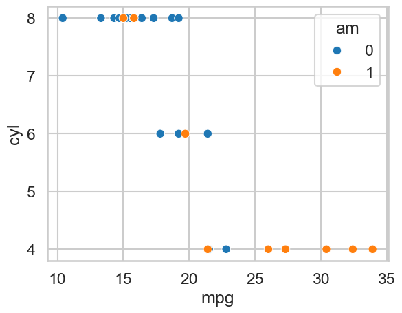
# produce a scatter plot of mpg against number of cylinders,
# but colour points by automatic/manual
sns.scatterplot(data=mtcars,
                x='mpg',
                y='cyl',
                hue='am')
<Axes: xlabel='mpg', ylabel='cyl'>
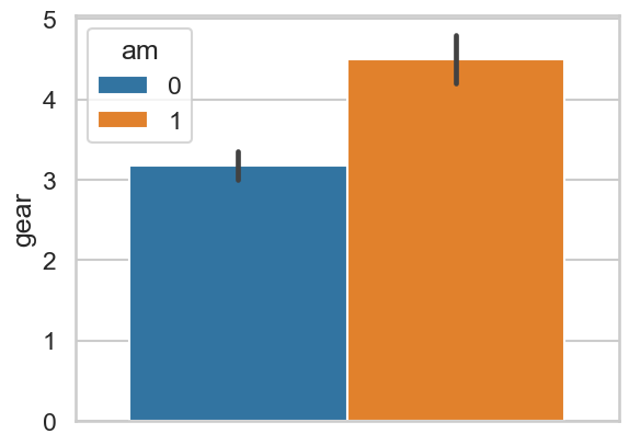
# Make a barplot of the number of gears for automatic/manual
sns.barplot(data=mtcars, y='gear', hue='am')
<Axes: ylabel='gear'>
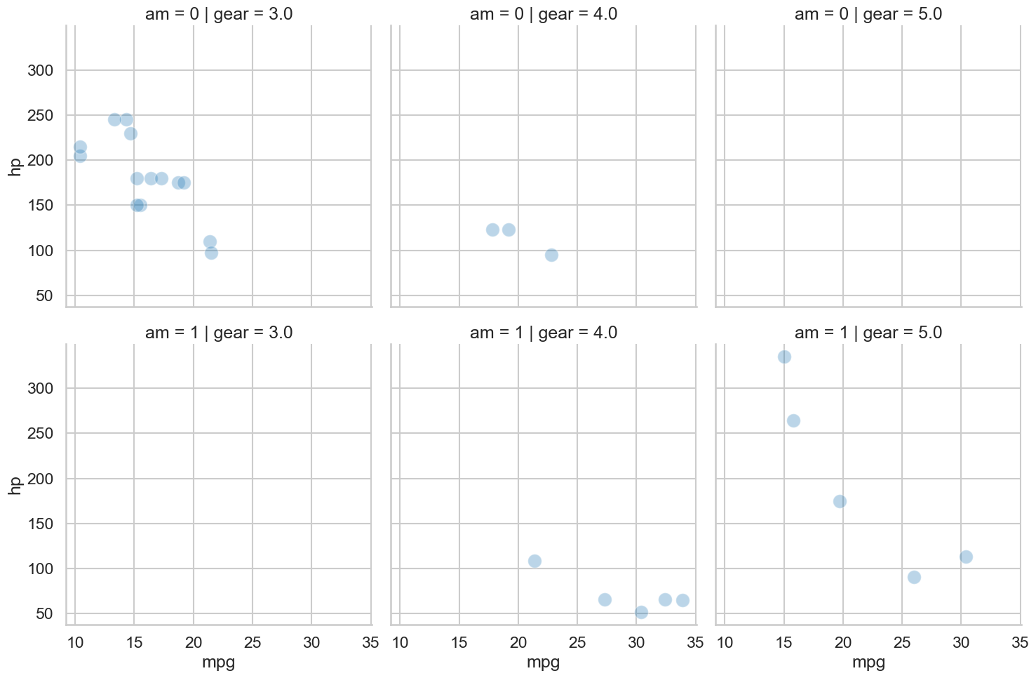
# Very complex plots can be made easily
# using the 'relplot' (for an association)
sns.relplot(data=mtcars,
            kind='scatter',
            row='am',
            col='gear',
            x='mpg', y='hp',
            s=200, alpha=.3);
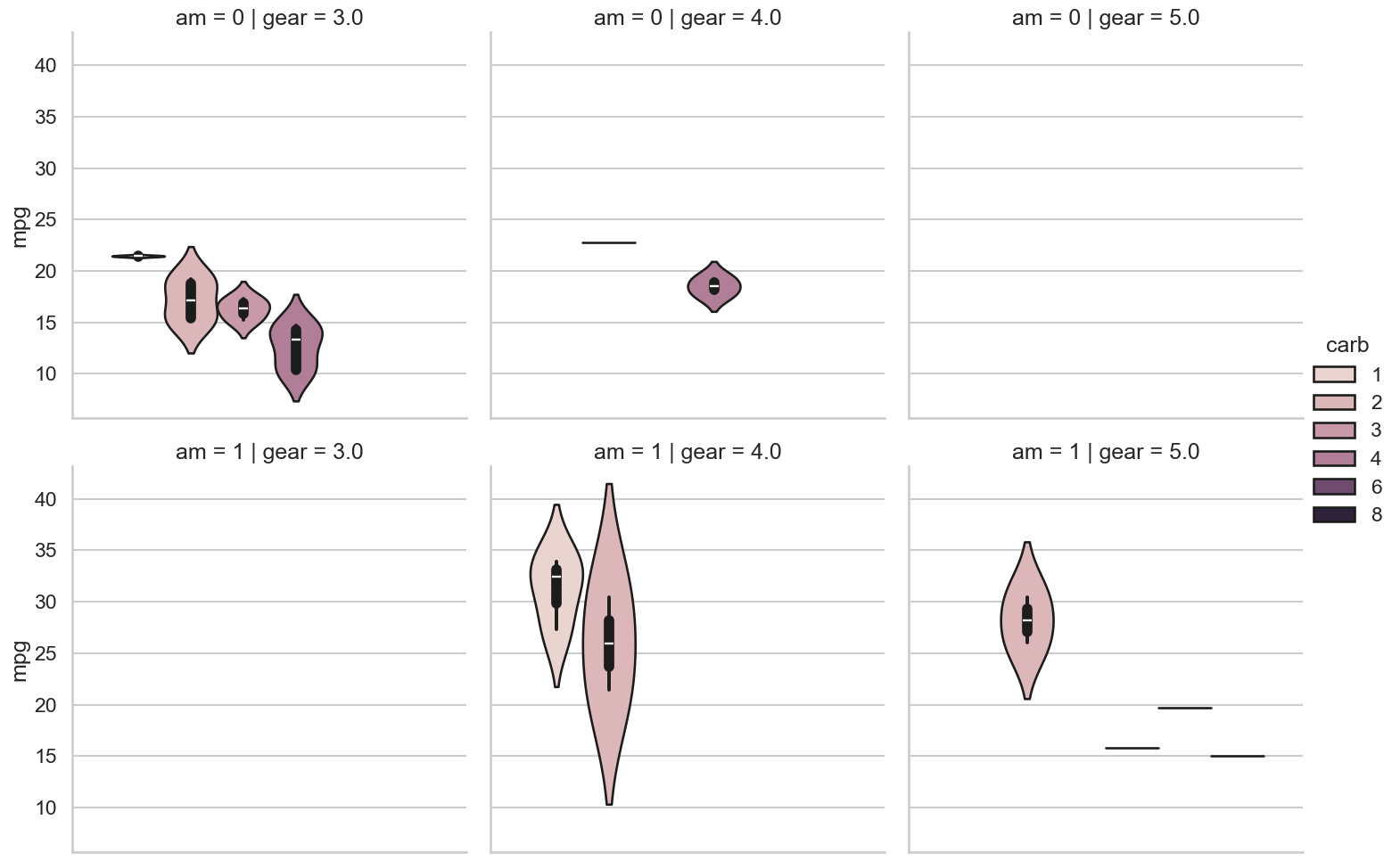
# ...or `catplot` for categorical data
sns.catplot(data=mtcars,
            kind='violin',
            row='am',
            col='gear',
            y='mpg', hue='carb');