Using Python for Data Analysis - Exercises & Answers#
1. Calculations in Python, and print#
For these exercises, try not to use Python. Instead, see if you can predict what would happen if you typed the commands into Python.
2 * 41 ** 310 / 510 % 9print(4 + 3)# print(9 / 3)
2. Variables and data types#
Again, try to imagine what would happen here. Then, try typing the commands to see if you were correct.
# Here are some some variables, whose values are used below.
a = 10
b = 5.789
c = '55'
d = True
type(a)b + ac - aprint('50 + 5 = ' + c)print('50 - ' + a '= 40)d + btype(b)c * 2 + c
3. Data Containers - the list#
Lists are an essential part of working with Python, being flexible, multipurpose containers for all kinds of data. The excercises below will require some coding on your part to fully answer the questions, and introduce some new topics and methods for lists not covered in the lecture material. As always with Python, exploring different options is the only way to really learn it.
When completing these exercises, you might make mistakes and modify the original data repeatedly. If that happens, clean up your code, and click Kernel -> Restart & Run All in the toolbar to start afresh.
a. Making a list#
First, define these variables:
age = 22; gender = 'M'; score_A = 459.321; score_B = 199.232
Now, store these in a list with the variable name my_list, in the order that they appear above.
Show code cell source
# First define variables
age = 22
gender = 'M'
score_A = 459.321
score_B = 199.232

# Then put into list
my_list = [age, gender, score_A, score_B]
print(my_list)
[22, 'M', 459.321, 199.232]
b. Accessing a list#
Print out the value 199.232 from my_list. What index position do you need to use?
Show code cell source
# Access this item with position number 3, or -1 (the last)
print(my_list[3], my_list[-1])
199.232 199.232
Use the .index method to find the index position of the letter ‘M’.
Show code cell source
# .index is easy
print(my_list.index('M'))
1
c. Complicated lists#
Define this rather long list:
long_list = [3, 8, [1, 2], 4, 4, 4, [99.234, 89.99, 45.322], ['junk'], 'final']
How would you access the value 89.99 in this list?
Show code cell source
# Its in the nested list in position 6, and then in THAT list its in position 1
long_list = [3, 8, [1, 2], 4, 4, 4, [99.234, 89.99, 45.322], ['junk'], 'final']
print(long_list[6][1])
89.99
4. Data Containers - the dictionary#
Dictionaries are also key parts of working with Python. You will also have to do some coding here to learn how they work, but hopefully you will find them intuitive.
a. Making a dictionary#
Make a dictionary, called dictionary_1, that has three entries. The first entry should have the key ‘a’, and the value ‘name’. The second entry should have the key ‘b’, and the value ‘age’. The third entry should have the key ‘c’, and the value [1, 2, 3] - so a list with the values 1, 2, 3.
Show code cell source
# Dictionary definition is easy
dictionary_1 = {'a': 'name', 'b': 'age', 'c': [1, 2, 3]}
b. Accessing values in a dictionary#
Now you have made a dictionary, how do you access the list with the values [1, 2, 3] in it? That is, what is the key for this and how do you use it?
Show code cell source
# With the key
print(dictionary_1['c'])
[1, 2, 3]
c. Adding a new key: value pair to a dictionary#
Can you add a new key value pair to the dictionary? The key should be ‘d’, and the value the string ‘final’.
Show code cell source
# Just like this
dictionary_1['d'] = 'final'
5. Using Pandas for some data analysis!#
Pandas is a vital part of working with data in Python. There are some exercises below to get you used to working with the package at a basic level.
a. Importing pandas#
You won’t get far without importing pandas. Write the traditional import statement for it below, which will allow you to use its functions and capability.
Show code cell source
# The classic import
import pandas as pd
b. Reading in a dataset#
Let us read a dataset in from the web. We will use the Palmer Penguins dataset, which is a real-life dataset of different penguin species on three different islands, containing mesaures of bill and flipper length, taken on different years, for male and female penguins (more here).
We will read this in directly from a location online, and explore some aspects of it using pandas.
The url for the dataset is here: https://raw.githubusercontent.com/mwaskom/seaborn-data/master/penguins.csv
Use pandas to read this in to a variable called penguins, and display the top and bottom 10 rows (head/tail) of the dataset.
Show code cell source
# Read straight from the internet like so
penguins = pd.read_csv('https://raw.githubusercontent.com/mwaskom/seaborn-data/master/penguins.csv')

# Head and tail
display(penguins.head(), penguins.tail())
| species | island | bill_length_mm | bill_depth_mm | flipper_length_mm | body_mass_g | sex | |
|---|---|---|---|---|---|---|---|
| 0 | Adelie | Torgersen | 39.1 | 18.7 | 181.0 | 3750.0 | MALE |
| 1 | Adelie | Torgersen | 39.5 | 17.4 | 186.0 | 3800.0 | FEMALE |
| 2 | Adelie | Torgersen | 40.3 | 18.0 | 195.0 | 3250.0 | FEMALE |
| 3 | Adelie | Torgersen | NaN | NaN | NaN | NaN | NaN |
| 4 | Adelie | Torgersen | 36.7 | 19.3 | 193.0 | 3450.0 | FEMALE |
| species | island | bill_length_mm | bill_depth_mm | flipper_length_mm | body_mass_g | sex | |
|---|---|---|---|---|---|---|---|
| 339 | Gentoo | Biscoe | NaN | NaN | NaN | NaN | NaN |
| 340 | Gentoo | Biscoe | 46.8 | 14.3 | 215.0 | 4850.0 | FEMALE |
| 341 | Gentoo | Biscoe | 50.4 | 15.7 | 222.0 | 5750.0 | MALE |
| 342 | Gentoo | Biscoe | 45.2 | 14.8 | 212.0 | 5200.0 | FEMALE |
| 343 | Gentoo | Biscoe | 49.9 | 16.1 | 213.0 | 5400.0 | MALE |
c. Checking data types#
Can you check what the data types of this penguin data has? What do you notice about the way the values look in the dataframe, and their types? What might an object data type mean?
Show code cell source
# Printing data types is easy
print(penguins.dtypes) # objects are basically 'strings'
species               object
island                object
bill_length_mm       float64
bill_depth_mm        float64
flipper_length_mm    float64
body_mass_g          float64
sex                   object
dtype: object
d. Checking and removing missing values#
Can you check whether there are missing values in the data? Which columns have missing data, and can you figure out how to count the number of missing values?
Once you have done this, do you think dropping or replacing the missing values is appropriate? Decide on an action and do it, storing the result in a new dataframe called clean_penguins.
Show code cell source
# Find the missing values like this
missing = penguins.isna() # this is the dataset where True == missing, False == present.

# then you can show which columns have any missing data
display(missing.any())

# You can count them like this
display(missing.sum()) # count per columns

# I would drop the missing values, so this
clean_penguins = penguins.dropna(how='any')
species              False
island               False
bill_length_mm        True
bill_depth_mm         True
flipper_length_mm     True
body_mass_g           True
sex                   True
dtype: bool
species               0
island                0
bill_length_mm        2
bill_depth_mm         2
flipper_length_mm     2
body_mass_g           2
sex                  11
dtype: int64
e. Querying some data#
In the new clean dataset, can you use describe after filtering the data to select these subsets?
Just male penguins?
Just Adelie penguins?
Penguins with a body mass above 4000 grams?
Adelie penguins on the Torgersen island?
Female penguins on the Biscoe or Torgerson island, with a body mass above 5000 grams?
Show code cell source
# For each of the queries you can do the following
# Males
males = clean_penguins.query('sex == "MALE"') # note the different quotations, you can mix them

# Adelie
adelie = clean_penguins.query('species == "Adelie"')

# Penguins with mass above 4000
chonks = clean_penguins.query('body_mass_g > 4000')

# On Torgensen and adelie
torgensen_adelie = clean_penguins.query('species == "Adelie" and island == "Torgenson"')

# Final one qhich is complex
# Note you can ask whether island is 'in' a list of options! Quite advanced.
complicated = clean_penguins.query('sex == "FEMALE" and island in ["Biscoe", "Torgerson"] and body_mass_g > 5000')

# Then you can use .describe on any of the above, e.g.
display(complicated.describe())
| bill_length_mm | bill_depth_mm | flipper_length_mm | body_mass_g | |
|---|---|---|---|---|
| count | 5.000000 | 5.000000 | 5.000000 | 5.000000 |
| mean | 46.160000 | 14.440000 | 213.800000 | 5140.000000 |
| std | 1.760114 | 0.650385 | 4.969909 | 65.192024 |
| min | 44.900000 | 13.300000 | 207.000000 | 5050.000000 |
| 25% | 45.100000 | 14.500000 | 212.000000 | 5100.000000 |
| 50% | 45.200000 | 14.800000 | 213.000000 | 5150.000000 |
| 75% | 46.500000 | 14.800000 | 217.000000 | 5200.000000 |
| max | 49.100000 | 14.800000 | 220.000000 | 5200.000000 |
f. Summarising data#
Here, we will compute some summary statistics from the penguins data, at both a single level (e.g., one column), and a grouped level. Remember the power of .agg here.
Can you compute the mean of the body mass variable?
What is the standard deviation of the bill length variable?
Using group-by, can you compute the mean body mass for males and females?
Taking it up a gear - can you compute the mean body mass for males and females, for all different species?
Finally, compute the mean, median, and counts for the body mass variable, for each sex, species, and island combination.
Show code cell source
# This heavily relies on .agg
# Mean body mass
mass = clean_penguins.agg({'body_mass_g': 'mean'})

# STD of bill
bill = clean_penguins.agg({'bill_length_mm': 'std'})

# Groupby males and females, aggregating mass
male_female_mass = clean_penguins.groupby(by=['sex']).agg({'body_mass_g': 'mean'})

# Same as above, but now including species
male_female_mass_species = clean_penguins.groupby(by=['sex', 'species']).agg({'body_mass_g': 'mean'})

# A big one, but made easy with the groupby and agg
complex_one = clean_penguins.groupby(by=['sex', 'species', 'island']).agg({'body_mass_g': ['mean', 'median', 'count']})
g. Reshaping data with some pop music#
Let us now advance a little bit to working with some bigger datasets and practicing reshaping. We’ll look at what is known as the billboard dataset, which contains all the songs that entered the billboard 100 during the year 2000 (retro I know), and their rankings at each of the recorded times.
First, go to the URL here: chendaniely/pandas_for_everyone
Download the dataset by clicking on the download icon. Once you have it, upload it to the server so you can read it.
Finally, read it into a variable called
billboard, and examine the head of it.
Show code cell source
# Read in easily enough once you have downloaded!
billboard = pd.read_csv('billboard.csv')

# Quite a large dataset here
billboard.head()
| year | artist | track | time | date.entered | wk1 | wk2 | wk3 | wk4 | wk5 | ... | wk67 | wk68 | wk69 | wk70 | wk71 | wk72 | wk73 | wk74 | wk75 | wk76 | |
|---|---|---|---|---|---|---|---|---|---|---|---|---|---|---|---|---|---|---|---|---|---|
| 0 | 2000 | 2 Pac | Baby Don't Cry (Keep... | 4:22 | 2000-02-26 | 87 | 82.0 | 72.0 | 77.0 | 87.0 | ... | NaN | NaN | NaN | NaN | NaN | NaN | NaN | NaN | NaN | NaN |
| 1 | 2000 | 2Ge+her | The Hardest Part Of ... | 3:15 | 2000-09-02 | 91 | 87.0 | 92.0 | NaN | NaN | ... | NaN | NaN | NaN | NaN | NaN | NaN | NaN | NaN | NaN | NaN |
| 2 | 2000 | 3 Doors Down | Kryptonite | 3:53 | 2000-04-08 | 81 | 70.0 | 68.0 | 67.0 | 66.0 | ... | NaN | NaN | NaN | NaN | NaN | NaN | NaN | NaN | NaN | NaN |
| 3 | 2000 | 3 Doors Down | Loser | 4:24 | 2000-10-21 | 76 | 76.0 | 72.0 | 69.0 | 67.0 | ... | NaN | NaN | NaN | NaN | NaN | NaN | NaN | NaN | NaN | NaN |
| 4 | 2000 | 504 Boyz | Wobble Wobble | 3:35 | 2000-04-15 | 57 | 34.0 | 25.0 | 17.0 | 17.0 | ... | NaN | NaN | NaN | NaN | NaN | NaN | NaN | NaN | NaN | NaN |
5 rows × 81 columns
Now you have the dataset, you can see it is a classic definition of a wide dataset. Each row contains many columns, in particular the rankings of each song at each week of the recorded timepoints. This is particularly annoying to work with, and what we could do is melt it into a long format.
Specifically, we want to keep the following columns as identifiers:
year,artist,track,time, anddate.entered.The rest (e.g.
wk1,wk2etc) are the value variables. You dont need to type all of them out. In fact, a clever trick is to simply not specify them, and pandas will know the ones you don’t specify inid_varswill be used as thevalue_vars.Can you set the name of the column capturing the questions to ‘week’ and the column capturing the score to
rank?
Store the result in a dataframe called billboard_long, and examine the head.
Show code cell source
# Melt billboard
billboard_long = billboard.melt(id_vars=['year', 'artist', 'track', 'time', 'date.entered'],
                                var_name='week', value_name='rank')

# Head
billboard_long.head()
| year | artist | track | time | date.entered | week | rank | |
|---|---|---|---|---|---|---|---|
| 0 | 2000 | 2 Pac | Baby Don't Cry (Keep... | 4:22 | 2000-02-26 | wk1 | 87.0 |
| 1 | 2000 | 2Ge+her | The Hardest Part Of ... | 3:15 | 2000-09-02 | wk1 | 91.0 |
| 2 | 2000 | 3 Doors Down | Kryptonite | 3:53 | 2000-04-08 | wk1 | 81.0 |
| 3 | 2000 | 3 Doors Down | Loser | 4:24 | 2000-10-21 | wk1 | 76.0 |
| 4 | 2000 | 504 Boyz | Wobble Wobble | 3:35 | 2000-04-15 | wk1 | 57.0 |
This format will allow easier interpretation and plotting. For example, computing the average rank for each song is much simpler in this format.
Finally for this - and without storing it anywhere, since you don’t need it - can you pivot the data back into its original form?
Show code cell source
# Pivot back wide
billboard_long.pivot(index=['year', 'artist', 'track', 'time', 'date.entered'],
                     columns='week', values='rank')
| week | wk1 | wk10 | wk11 | wk12 | wk13 | wk14 | wk15 | wk16 | wk17 | wk18 | ... | wk7 | wk70 | wk71 | wk72 | wk73 | wk74 | wk75 | wk76 | wk8 | wk9 | ||||
|---|---|---|---|---|---|---|---|---|---|---|---|---|---|---|---|---|---|---|---|---|---|---|---|---|---|
| year | artist | track | time | date.entered | |||||||||||||||||||||
| 2000 | 2 Pac | Baby Don't Cry (Keep... | 4:22 | 2000-02-26 | 87.0 | NaN | NaN | NaN | NaN | NaN | NaN | NaN | NaN | NaN | ... | 99.0 | NaN | NaN | NaN | NaN | NaN | NaN | NaN | NaN | NaN |
| 2Ge+her | The Hardest Part Of ... | 3:15 | 2000-09-02 | 91.0 | NaN | NaN | NaN | NaN | NaN | NaN | NaN | NaN | NaN | ... | NaN | NaN | NaN | NaN | NaN | NaN | NaN | NaN | NaN | NaN | |
| 3 Doors Down | Kryptonite | 3:53 | 2000-04-08 | 81.0 | 51.0 | 51.0 | 51.0 | 47.0 | 44.0 | 38.0 | 28.0 | 22.0 | 18.0 | ... | 54.0 | NaN | NaN | NaN | NaN | NaN | NaN | NaN | 53.0 | 51.0 | |
| Loser | 4:24 | 2000-10-21 | 76.0 | 61.0 | 61.0 | 59.0 | 61.0 | 66.0 | 72.0 | 76.0 | 75.0 | 67.0 | ... | 55.0 | NaN | NaN | NaN | NaN | NaN | NaN | NaN | 59.0 | 62.0 | ||
| 504 Boyz | Wobble Wobble | 3:35 | 2000-04-15 | 57.0 | 57.0 | 64.0 | 70.0 | 75.0 | 76.0 | 78.0 | 85.0 | 92.0 | 96.0 | ... | 36.0 | NaN | NaN | NaN | NaN | NaN | NaN | NaN | 49.0 | 53.0 | |
| ... | ... | ... | ... | ... | ... | ... | ... | ... | ... | ... | ... | ... | ... | ... | ... | ... | ... | ... | ... | ... | ... | ... | ... | ... | |
| Yankee Grey | Another Nine Minutes | 3:10 | 2000-04-29 | 86.0 | NaN | NaN | NaN | NaN | NaN | NaN | NaN | NaN | NaN | ... | 88.0 | NaN | NaN | NaN | NaN | NaN | NaN | NaN | 95.0 | NaN | |
| Yearwood, Trisha | Real Live Woman | 3:55 | 2000-04-01 | 85.0 | NaN | NaN | NaN | NaN | NaN | NaN | NaN | NaN | NaN | ... | NaN | NaN | NaN | NaN | NaN | NaN | NaN | NaN | NaN | NaN | |
| Ying Yang Twins | Whistle While You Tw... | 4:19 | 2000-03-18 | 95.0 | 89.0 | 97.0 | 96.0 | 99.0 | 99.0 | NaN | NaN | NaN | NaN | ... | 74.0 | NaN | NaN | NaN | NaN | NaN | NaN | NaN | 78.0 | 85.0 | |
| Zombie Nation | Kernkraft 400 | 3:30 | 2000-09-02 | 99.0 | NaN | NaN | NaN | NaN | NaN | NaN | NaN | NaN | NaN | ... | NaN | NaN | NaN | NaN | NaN | NaN | NaN | NaN | NaN | NaN | |
| matchbox twenty | Bent | 4:12 | 2000-04-29 | 60.0 | 12.0 | 8.0 | 6.0 | 1.0 | 2.0 | 3.0 | 2.0 | 2.0 | 3.0 | ... | 18.0 | NaN | NaN | NaN | NaN | NaN | NaN | NaN | 16.0 | 13.0 |
317 rows × 76 columns
There is no ‘right’ data format. But some formats are more amenable to computing certain statistics, others for plotting, and others for presenting to collaborators, viewing, etc. You have to know how to go between the two.
6. Plotting#
We come to the last set of exercises now, where we will attempt some simple plots. First, let us import seaborn, and if you want, you can use the other bits of code I wrote to alter the appearance of the plots!
Import seaborn with its usual alias below. If you like, add extra code to alter the visualisations.
Show code cell source
# Import seaborn and set plotting appearance
import seaborn as sns # traditionally as `sns`

# These lines are optional, but make our plots look nicer!
sns.set_style('whitegrid')
sns.set_context('talk')
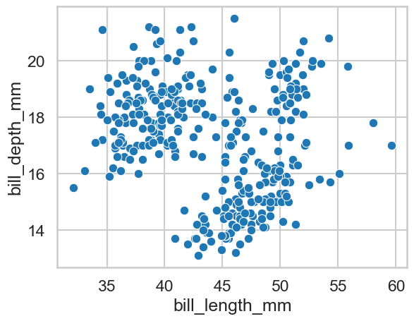
a. Plotting some penguin bills#
We will rely on our clean_penguins dataset for this, and you should also have open in browser the Seaborn Gallery, which will tell you the many commands to produce plots.
First, can you do a simple scatterplot of bill length against bill depth?
Show code cell source
# Plot like so
sns.scatterplot(data=clean_penguins, x='bill_length_mm', y='bill_depth_mm')
<Axes: xlabel='bill_length_mm', ylabel='bill_depth_mm'>
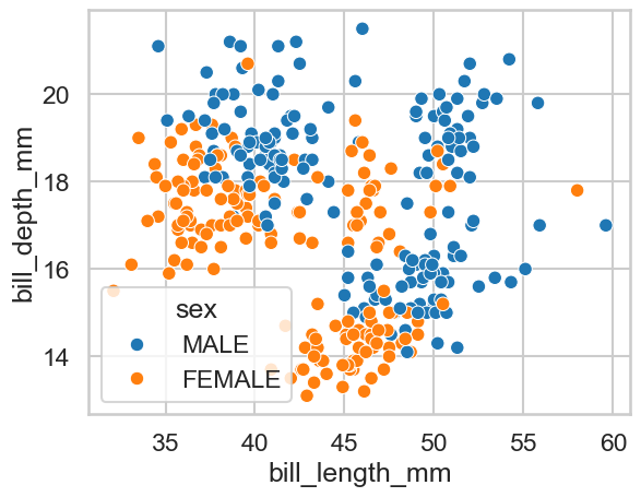
b. Expanding our plots of penguins#
Can you modify the answer to part a to alter the colour of the markers so they reveal whether the observation belongs to a female or a male penguin?
Show code cell source
# Plot like so - add 'hue', and set it to sex
sns.scatterplot(data=clean_penguins, x='bill_length_mm', y='bill_depth_mm', hue='sex')
<Axes: xlabel='bill_length_mm', ylabel='bill_depth_mm'>
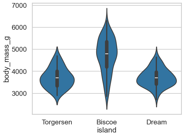
c. Violins and penguins#
Can you now produce a plot that shows the body mass of penguins at each island, in the form of a violin plot - see the example gallery if you are stuck!
Show code cell source
# Violins like this
sns.violinplot(data=clean_penguins, x='island', y='body_mass_g')
<Axes: xlabel='island', ylabel='body_mass_g'>
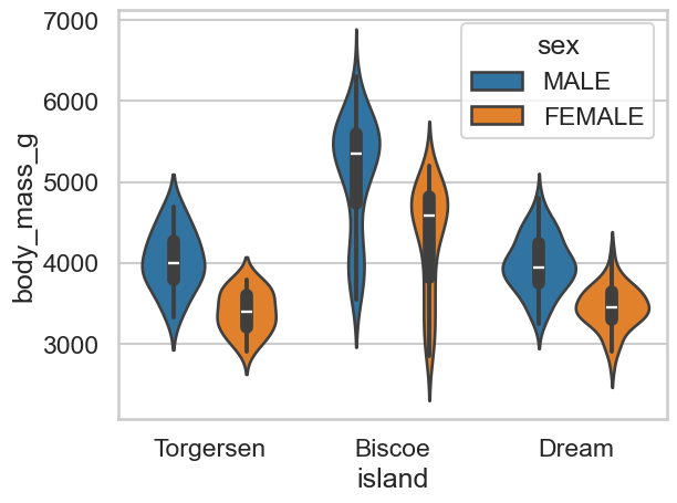
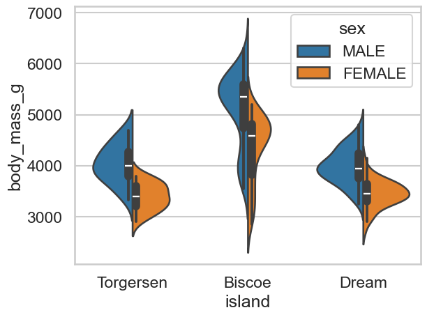
d. More violins and penguins#
Expand the previous answer so you show the two different sexes for each island in your violin plot. You may need to use the
splitargument in your command.
Show code cell source
# Add sex in like this
sns.violinplot(data=clean_penguins, x='island', y='body_mass_g', hue='sex')
<Axes: xlabel='island', ylabel='body_mass_g'>
Show code cell source
# Add sex in like this, you can also split
sns.violinplot(data=clean_penguins, x='island', y='body_mass_g', hue='sex', split=True)
<Axes: xlabel='island', ylabel='body_mass_g'>
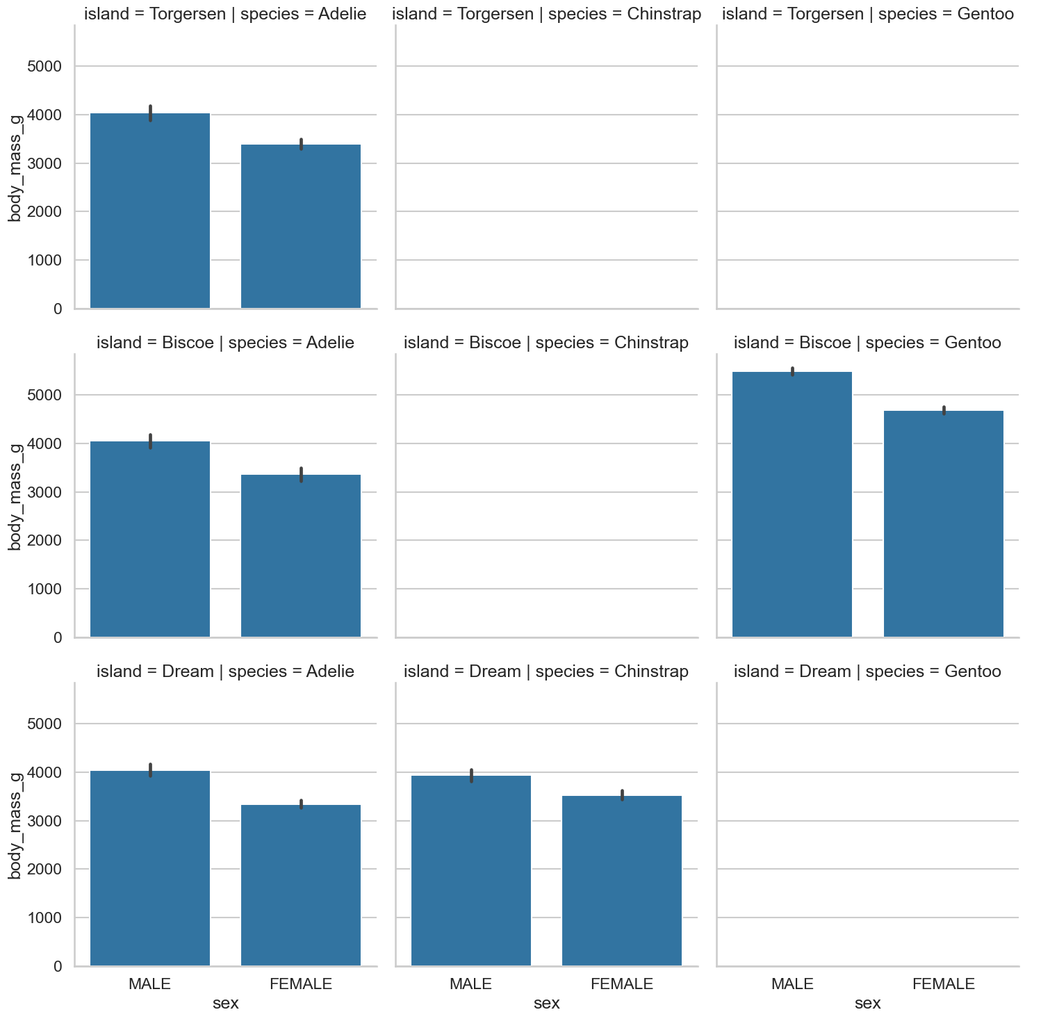
e. Cat(plots) and penguins#
Lets take it up to as much complexity as we can handle. Using a
catplot, produce a plot that has, for each island and penguin species, a bar chart for body mass between the sexes. You should end up with a 3 x 3 grid of plots.Why are some of these empty?
Show code cell source
# Sounds hard, but its not so bad
sns.catplot(data=clean_penguins,
            kind='bar',
            x='sex',
            y='body_mass_g',
            row='island',
            col='species')
<seaborn.axisgrid.FacetGrid at 0x13120e410>
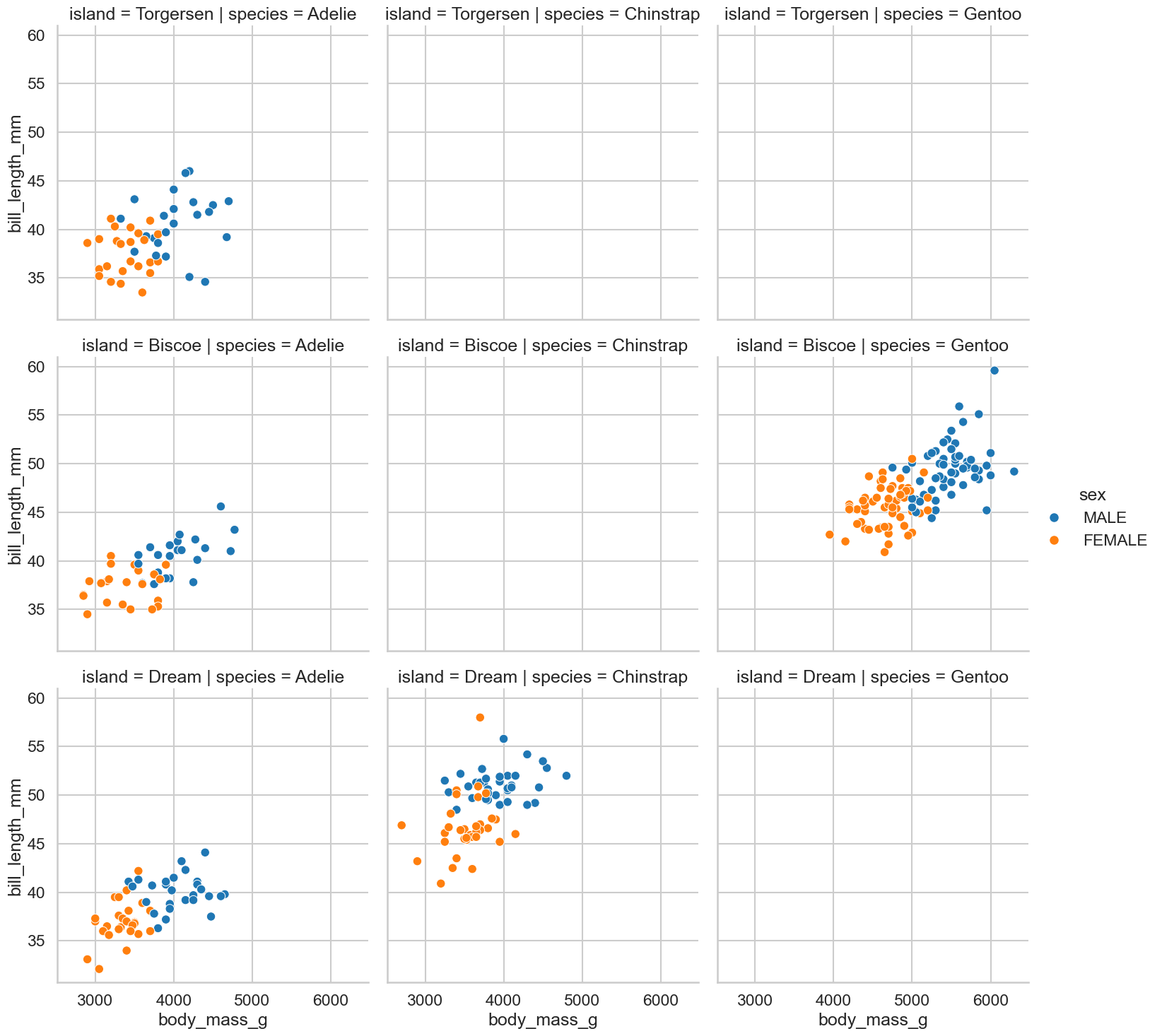
f. Relplots#
A final challenge. Can you produce a scatterplot that plots body mass against bill length, and has different colours for each sex, and has a separate plot for each combination of species and island locations? If you use
relplotthis should not be as hard as it might sound!Can you figure out again why some of these are empty?
Show code cell source
# Similar to the above, but using relplot
sns.relplot(data=clean_penguins,
            kind='scatter',
            x='body_mass_g',
            y='bill_length_mm',
            hue='sex',
            row='island',
            col='species')
<seaborn.axisgrid.FacetGrid at 0x1315bf510>