Statistics with statsmodels and scipy.stats
Contents
2. Statistics with statsmodels and scipy.stats#
Python has two mature and powerful packages for statistical inference that are general in nature - scipy and statsmodels. In fact, pingouin relies pretty much entirely on these packages for behind-the-scenes computation. Nothing beats diving into the details, so this section will take a close look at these packages.
statsmodelsallows users to fit a wide range of general and generalized linear models, random effects models, general additive models, and more. Often, one can fit these models using a “formula” style syntax that is inspired byR. As your statistical knowledge and comfort grows, you will want to progress to using this module as it is fully flexible - for example, it can estimate ordinal or Poisson regression models, whichpingouincannot. I find I usestatsmodelsdaily.scipy, and in particular its.statssubmodule, contain a range of useful statistical functions likezscore,pearsonr, and many more, as well as carrying a range of statistical distributions that allow you to estimate the probability of data in a clean and straightforward way.
We will examine statsmodels in some detail here, in particular the workhorse of statistical inference - ordinary least squares, which is heavily used in psychology and beyond to estimate linear models.
2.1. statsmodels - introduction to ordinary least squares and the formula interface#
Ordinary least squares fits a line to data - a so-called linear model. The slope and intercepts of those lines can be use to make inferences about the relationship between variables.
statsmodels allows you to specify those relationships with a formula string. The formula interface to statsmodels is imported as smf. An example will make things clearer, using the crash dataset from the previous example. Lets load up the usual packages in addition to statsmodels.
import numpy as np
import pandas as pd
import pingouin as pg
import matplotlib.pyplot as plt
import seaborn as sns
import statsmodels.formula.api as smf # the formula interface of statsmodels

crash = sns.load_dataset('car_crashes')
/Users/alexjones/opt/anaconda3/envs/py10/lib/python3.10/site-packages/outdated/utils.py:14: OutdatedPackageWarning: The package pingouin is out of date. Your version is 0.5.1, the latest is 0.5.2.
Set the environment variable OUTDATED_IGNORE=1 to disable these warnings.
  return warn(
# Lets say we want to predict ins_losses from speeding, alcohol, and ins_premium
formula = 'ins_losses ~ 1 + speeding + alcohol + ins_premium'
This formula specifies that we predicting ins_losses from the additive model of speeding, alcohol, and ins_premium variables. Starting the formula a ‘1 +’ simply means to compute a intercept. To build this model, we first need to pass it to the ols class from statsmodels and give it the associated data, and store it in a variable. Then, we need to call the .fit() method on this model - this will actually carry out the maths behind regression. Its easy to do this in one step. Once done, we can access the .summary() method and look at the model. statsmodels produces an in-depth output that contains all the data we need for analysis - particularly the coefficients, \(R^2\), \(F\) values, and degrees of freedom.
# Build a model and fit it at the same time.
model = smf.ols(formula, data=crash).fit()

# Examine the results
model.summary()
| Dep. Variable: | ins_losses | R-squared: | 0.389 |
|---|---|---|---|
| Model: | OLS | Adj. R-squared: | 0.350 |
| Method: | Least Squares | F-statistic: | 9.959 |
| Date: | Sat, 09 Jul 2022 | Prob (F-statistic): | 3.40e-05 |
| Time: | 11:56:55 | Log-Likelihood: | -223.14 |
| No. Observations: | 51 | AIC: | 454.3 |
| Df Residuals: | 47 | BIC: | 462.0 |
| Df Model: | 3 | ||
| Covariance Type: | nonrobust |
| coef | std err | t | P>|t| | [0.025 | 0.975] | |
|---|---|---|---|---|---|---|
| Intercept | 58.3212 | 17.892 | 3.260 | 0.002 | 22.327 | 94.315 |
| speeding | -0.2978 | 1.893 | -0.157 | 0.876 | -4.106 | 3.510 |
| alcohol | 0.1428 | 2.235 | 0.064 | 0.949 | -4.353 | 4.639 |
| ins_premium | 0.0868 | 0.016 | 5.375 | 0.000 | 0.054 | 0.119 |
| Omnibus: | 0.929 | Durbin-Watson: | 2.253 |
|---|---|---|---|
| Prob(Omnibus): | 0.629 | Jarque-Bera (JB): | 0.953 |
| Skew: | 0.297 | Prob(JB): | 0.621 |
| Kurtosis: | 2.689 | Cond. No. | 5.78e+03 |
Notes:
[1] Standard Errors assume that the covariance matrix of the errors is correctly specified.
[2] The condition number is large, 5.78e+03. This might indicate that there are
strong multicollinearity or other numerical problems.
statsmodels produces an in-depth output that contains all the data we need for analysis - particularly the coefficients, \(R^2\), \(F\) values, and degrees of freedom, as well as other kinds of model fit such as \(AIC\) - Akaike’s Information Criterion, as well as \(BIC\), the Bayesian Information Criterion.
2.1.1. The ResultsWrapper object#
A fitted regression model, like the model variable above, is a special type of object from statsmodels called a ResultsWrapper:
type(model)
statsmodels.regression.linear_model.RegressionResultsWrapper
This object has a range of extremely useful attributes. For example, it contains the .fittedvalues and .resid attributes, which are the predicted values, and residuals (observed - predicted), respectively. Both are stored as pandas Series objects (one-dimensional DataFrames).
# Get predicted
display(model.fittedvalues.head())

# Get errors
display(model.resid.head())
0    125.019442
1    148.169326
2    135.174427
3    129.741571
4    133.771227
dtype: float64
0    20.060558
1   -14.239326
2   -24.824427
3    12.648429
4    31.858773
dtype: float64
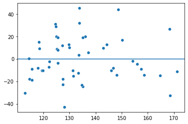
This makes it very easy to check model assumptions graphically:
# Check residual plot of errors against predictions
plot = sns.scatterplot(x=model.fittedvalues, y=model.resid)
plot.axhline(0)
<matplotlib.lines.Line2D at 0x12d453d00>
The ResultsWrapper contains a range of other useful attributes and methods, including robust covariances and tests for linear parameter contrasts. For example, we can test whether the alcohol coefficient is different from .10, and whether the ins_premium and alcohol coefficients are significantly different, using the .t_test method, as well as a formula string describing our tests:
model.t_test('ins_premium = alcohol, alcohol = .10')
<class 'statsmodels.stats.contrast.ContrastResults'>
                             Test for Constraints
==============================================================================
                 coef    std err          t      P>|t|      [0.025      0.975]
------------------------------------------------------------------------------
c0            -0.0560      2.232     -0.025      0.980      -4.547       4.435
c1             0.1428      2.235      0.019      0.985      -4.353       4.639
==============================================================================
2.1.2. Prediction Objects#
The ResultsWrapper object also has a very helpful method named .get_prediction. This allows for inference on either the fitted data (call the method without any arguments) or on new, held out data (pass the DataFrame with the data to the method).
The method returns a PredictionResults object, which contains the predicted values as well as their uncertainty in terms of the confidence intervals around both the average prediction and the prediction interval (where new observed values may fall).
The PredictionResults object has a further method, .summary_frame, which will return the data in a DataFrame. Let’s get the predictions of the insurance losses we modelled above, for the in-sample data:
# Get the in-sample predictions
in_sample_predictions = model.get_prediction().summary_frame()
display(in_sample_predictions.head())
| mean | mean_se | mean_ci_lower | mean_ci_upper | obs_ci_lower | obs_ci_upper | |
|---|---|---|---|---|---|---|
| 0 | 125.019442 | 4.779806 | 115.403713 | 134.635170 | 83.594182 | 166.444702 |
| 1 | 148.169326 | 6.308884 | 135.477489 | 160.861163 | 105.923940 | 190.414712 |
| 2 | 135.174427 | 3.722046 | 127.686636 | 142.662218 | 94.190809 | 176.158045 |
| 3 | 129.741571 | 4.563009 | 120.561981 | 138.921161 | 88.415371 | 171.067771 |
| 4 | 133.771227 | 3.879437 | 125.966807 | 141.575648 | 92.728580 | 174.813875 |
There is a row for each observation. The mean column represents the prediction, and is identical to the .fittedvalues data. The mean_se is an estimate of the standard error of each prediction, and the ci columns represent the confidence interval around the mean. The obs_ci represents something different, the interval for within which new data points would be expected to fall (not the average).
2.1.3. Marginal predictions or counterfactuals#
Lets take this a step further and explore the elegance of modelling for examining statistical relationships. We can explore the marginal predictions of variables by “holding constant” others, and use the tools we’ve seen above to get some uncertainty around this. Imagine that we are interested in the relationship between insurance premiums and insurance losses in accidents, while we account for speeding and alcohol. ins_premium was our only significant predictor in our model above (check model.summary() for a refresher), and we can examine what this looks like.
To do this, we need to take our fitted model and have it predict a ‘counterfactual’ world, where insurance premium varies but alcohol and speeding are held at some particular value. This ‘particular value’ can be anything we want, but it is typically the mean of a predictor variable. Below, we will ask the model to predict the insurance loss for the observed insurance premium data, but we will fix alcohol and speeding to be at their mean. Doing so with pandas is easy:
# Make a 'new' dataset to predict:
new_data = (crash
            .filter(items=['ins_losses', 'ins_premium']) # gets the existing data columns
            .assign(alcohol = crash['alcohol'].mean(),
                    speeding = crash['speeding'].mean())
           )

new_data.head()
| ins_losses | ins_premium | alcohol | speeding | |
|---|---|---|---|---|
| 0 | 145.08 | 784.55 | 4.886784 | 4.998196 |
| 1 | 133.93 | 1053.48 | 4.886784 | 4.998196 |
| 2 | 110.35 | 899.47 | 4.886784 | 4.998196 |
| 3 | 142.39 | 827.34 | 4.886784 | 4.998196 |
| 4 | 165.63 | 878.41 | 4.886784 | 4.998196 |
So we have a new dataset with the same insurance loss and insurance premium as before, but now we’re imagining a world in which all the accidents took place where alcohol use was average, and speeding was also average. Note that these column names here must reflect the original column names used in the model fitting stage, or it will not work.
We next pass this data to the get_prediction method, and we immediately call the summary_frame method to get the predictions formatted nicely:
# Get new predictions
new_predictions = model.get_prediction(new_data).summary_frame()
new_predictions.head()
| mean | mean_se | mean_ci_lower | mean_ci_upper | obs_ci_lower | obs_ci_upper | |
|---|---|---|---|---|---|---|
| 0 | 125.607033 | 3.255652 | 119.057505 | 132.156561 | 84.784414 | 166.429652 |
| 1 | 148.942596 | 3.884950 | 141.127084 | 156.758108 | 107.897838 | 189.987353 |
| 2 | 135.578858 | 2.811930 | 129.921984 | 141.235732 | 94.889914 | 176.267801 |
| 3 | 129.320002 | 2.965204 | 123.354781 | 135.285222 | 88.587045 | 170.052959 |
| 4 | 133.751442 | 2.808058 | 128.102357 | 139.400526 | 93.063580 | 174.439303 |
It would be great to plot this data, but one tricky extra step is that plotting is made easier by sorting the predictions by the predictor of interest. One way to do this is to join everything into one dataset (the new data and the predictions) and plot that, like so:
# Join data together
new_predictions = pd.merge(left=new_data, right=new_predictions,
                           left_index=True, right_index=True).sort_values(by='ins_premium')
# Use context manager
with sns.plotting_context('talk'):

    fig, ax = plt.subplots(1, 1, figsize=(10, 10))
    sns.despine(fig)

    # Seaborn lineplot to show the relationship
    sns.lineplot(x=new_predictions['ins_premium'],
                 y=new_predictions['mean'],
                 linestyle='dashed',
                 linewidth=4,
                 color='black',
                 ax=ax)

    # Fill between is an axis method that shades an area between two Y and one X dataset
    ax.fill_between(new_predictions['ins_premium'],
                    new_predictions['mean_ci_lower'],
                    new_predictions['mean_ci_upper'],
                    alpha=.1,
                    color='red',
                    label='Mean CI')

    ax.fill_between(new_predictions['ins_premium'],
                    new_predictions['obs_ci_lower'],
                    new_predictions['obs_ci_upper'],
                    alpha=.1,
                    color='blue',
                    label='Prediction CI')

    ax.legend() # show legend
    ax.set(ylabel='Predicted Insurance Loss $', xlabel='Insurance Premium $') # Set labels
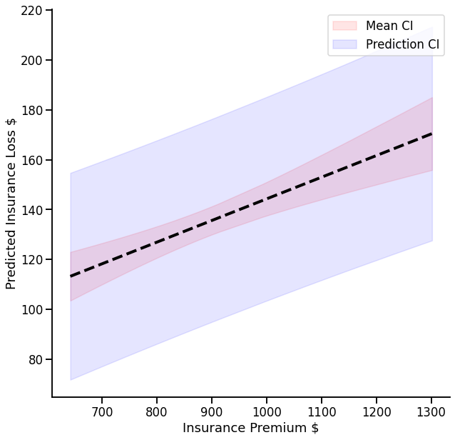
There is a positive relationship here - accounting for speeding and alcohol, accidents with higher premiums result in greater losses. There is some greater uncertainty about the mean of this relationship at the extreme ends of the ins_premium variable; but its quite focused. The prediction intervals on the other hand are much wider - the model implies that, for example, an accident with a $900 premium (and, don’t forget - average speeding and average alcohol use!) could lose anywhere between ~95 and ~170.