Generalised Linear Models
Contents
# Imports
import numpy as np
import pandas as pd
import seaborn as sns
import matplotlib.pyplot as plt
import statsmodels.formula.api as smf
3. Generalised Linear Models#
statsmodels is far more than a linear regression powerhouse. It is also capable of fitting a range of generalised linear models, that allow users to fit models to non-normal data, such as binary, count, hierarchical models, and generalised estimating equations. We will explore some of these using the in-built datasets from statsmodels. These are located under the non-formula import of the package, which exposes a far wider range of functions outside of the nice formula interface we have seen so far.
# Import general statsmodels
import statsmodels.api as sm # traditional alias
3.1. Logistic Regression#
We will first explore the use of logistic regression, which allows for the modelling of binary data - such as whether a trial was correct/incorrect, a participant was male/female, and so on. For this example we will use the RAND Health Insurance Experiment data which contains a set of variables related to health insurance claims that have been used to investigate key questions in health insurance. The variables are:
mdvis- Number of outpatient visits to an MDlncoins- ln(coinsurance + 1), 0 <= coninsurance <= 10idp- 1 if individual deductible plan, 0 otherwiselpi- ln(max(1, annual participation incentive payment)fmde- 0 if idp = 1; ln(max(1, MDE/(0.01 coinsurance))) otherwisephyslm- 1 if the person has a physical limitationdisea- number of chronic diseasehlthg- 1 if self-rated health is goodhlthf- 1 if self-rated health is fairhlthp- 1 if self-rated health is poor
We will attempt a simple logistic regression model, predicting whether someone has an individual deductible plan, idp (coded as 1 if yes, and zero if no) from a few predictors - number of chronic diseases disea, number of outpatient visits mdvis, and coinsurance, the amount that has to be paid if a claim is made, lncoins.
To fit logistic regression models, we can use the logit function from the formula smf interface, and specify our model with a formula string. But first we load the data (with a slightly unusual syntax) from the non-formula interface:
# Load RAND data
rand = sm.datasets.randhie.load_pandas().data

# Fit the model
logistic_results = smf.logit('idp ~ disea + mdvis + lncoins', data=rand).fit()

# Examine the results
logistic_results.summary()
Optimization terminated successfully.
         Current function value: 0.537159
         Iterations 6
| Dep. Variable: | idp | No. Observations: | 20190 |
|---|---|---|---|
| Model: | Logit | Df Residuals: | 20186 |
| Method: | MLE | Df Model: | 3 |
| Date: | Sat, 09 Jul 2022 | Pseudo R-squ.: | 0.06261 |
| Time: | 11:56:15 | Log-Likelihood: | -10845. |
| converged: | True | LL-Null: | -11570. |
| Covariance Type: | nonrobust | LLR p-value: | 0.000 |
| coef | std err | z | P>|z| | [0.025 | 0.975] | |
|---|---|---|---|---|---|---|
| Intercept | -0.5700 | 0.034 | -16.585 | 0.000 | -0.637 | -0.503 |
| disea | 0.0122 | 0.003 | 4.865 | 0.000 | 0.007 | 0.017 |
| mdvis | -0.0495 | 0.005 | -10.399 | 0.000 | -0.059 | -0.040 |
| lncoins | -0.3259 | 0.009 | -34.907 | 0.000 | -0.344 | -0.308 |
Success! But what does all this mean? Logistic regression isn’t as easy to interpret as ordinary least squares, where a single unit increase in the predictor is associated with a coefficient-value change in the outcome. Logistic regression actually models the probability of a positive/yes/one response in the outcome variable, but does so using the logistic function, which maps probability space, which is zero to one, to an infinite continuous space of positive and negative.
The way it does this is by converting probabilities to odds, and then taking the logarithm of the odds - the log-odds. All coefficients in logistic regression represent the change in the log-odds of the outcome with a one-unit increase of the predictor.
Let’s try to clear this up by looking at the model. The mdvis predictor shows a significant, negative relationship with the outcome on the log-odds scale. We have no idea what this means outside of that when the number of visits go up, the probability of having a deductible plan goes down. But if we exponentiate the coefficient, we undo the logarithm and get the odds back, which are somewhat more interpretable. numpy can help us here!
# Use numpy to exponentiate the coefficients
# numpy has an .exp function
# the coefficients are stored in the .params model attribute
odds = np.exp(logistic_results.params)
odds
Intercept    0.565516
disea        1.012295
mdvis        0.951673
lncoins      0.721882
dtype: float64
This is somewhat more interpretable. As the number of medical visits increases by one, the odds of having an individual deductible plan change by 0.95% (or indeed decrease by 5%).
Unlike ordinary least squares, understanding a logistic regression model involves working closely with the predictions. We saw how to get those from an ols object above, but logistic regression is a different beast. While it does have a .fittedvalues attribute, it represents the predictions on the log-odds scale. To get at our predictions, we can do two things:
Apply the reverse transformation using
scipy.special.expiton the.fittedvaluesattribute. This is the inverse-log-odds transform (sometimes known as the inverse logit) and will return the probabilities of a positive response.Use the
.predictmethod of the fitted model to give the probabilites already back-transformed.
The latter doesn’t invovle an extra import but we will show both:
# import scipy function
from scipy.special import expit
expit_results = expit(logistic_results.fittedvalues)

# Use prediction
logistic_predictions = logistic_results.predict() # a no-argument call predicts the data the model was fitted on

# Are these the same?
np.all(expit_results == logistic_predictions)
True
These are equivalent operations. Let’s work with the logistic_predictions data, and add it directly to the rand data.
# add a column
rand['predictions'] = logistic_results.predict()

display(rand.head())
| mdvis | lncoins | idp | lpi | fmde | physlm | disea | hlthg | hlthf | hlthp | predictions | |
|---|---|---|---|---|---|---|---|---|---|---|---|
| 0 | 0 | 4.61512 | 1 | 6.907755 | 0.0 | 0.0 | 13.73189 | 1 | 0 | 0 | 0.129403 |
| 1 | 2 | 4.61512 | 1 | 6.907755 | 0.0 | 0.0 | 13.73189 | 1 | 0 | 0 | 0.118646 |
| 2 | 0 | 4.61512 | 1 | 6.907755 | 0.0 | 0.0 | 13.73189 | 1 | 0 | 0 | 0.129403 |
| 3 | 0 | 4.61512 | 1 | 6.907755 | 0.0 | 0.0 | 13.73189 | 1 | 0 | 0 | 0.129403 |
| 4 | 0 | 4.61512 | 1 | 6.907755 | 0.0 | 0.0 | 13.73189 | 1 | 0 | 0 | 0.129403 |
Our model has given us the predictions of whether someone has an individual deductible plan. If you’re not used to logistic regression it may be a surprise that you get probabilities back and not zeros and ones, which is what you have in the observed data. Its actually entirely up to you how you interpret those probabilities and to map them onto the observed data, but its tradition that we assume the outcome variable is a \(Bernoulli\) distributed variable (stats speak for functioning like a coin toss with heads-tails outcomes, which we want to know the probability of heads). We can actually convert the probabilities into zeros and ones with a simple boolean operation, sometimes known as thresholding:
# add zeros/ones
rand['predicted_idp'] = np.where(rand['predictions'] <= .50, 0, 1)

rand.head()
| mdvis | lncoins | idp | lpi | fmde | physlm | disea | hlthg | hlthf | hlthp | predictions | predicted_idp | |
|---|---|---|---|---|---|---|---|---|---|---|---|---|
| 0 | 0 | 4.61512 | 1 | 6.907755 | 0.0 | 0.0 | 13.73189 | 1 | 0 | 0 | 0.129403 | 0 |
| 1 | 2 | 4.61512 | 1 | 6.907755 | 0.0 | 0.0 | 13.73189 | 1 | 0 | 0 | 0.118646 | 0 |
| 2 | 0 | 4.61512 | 1 | 6.907755 | 0.0 | 0.0 | 13.73189 | 1 | 0 | 0 | 0.129403 | 0 |
| 3 | 0 | 4.61512 | 1 | 6.907755 | 0.0 | 0.0 | 13.73189 | 1 | 0 | 0 | 0.129403 | 0 |
| 4 | 0 | 4.61512 | 1 | 6.907755 | 0.0 | 0.0 | 13.73189 | 1 | 0 | 0 | 0.129403 | 0 |
We can now examine how well the model did in terms of its predictions, by computing the terrifyingly named confusion matrix. All this represents is how our model did - for example, when a datapoint did have an individual deductible, how many times did the model say it did? What about the reverse - did it say no when it should have said no?
Evaluating the performance of logistic regression models is an entire sub-field of statistics in and of itself. You will sometime see terms like precision, recall, accuracy, true positive rate, false positive rate, and many, many more floating around. All of these refer to - basically - is whether the model is saying ‘yes’ when it should and ‘no’ when it should, and there are many variations along that theme. Personally I find this the most confusing part of statistical practice and find myself always referring to this diagram when working here - I am sure you will too!
Let’s use the pd.crosstab function to build the confusion matrix, which takes two columns of 1/0 responses and counts the values:
# Crosstabs can be normalised or not, depending on the use of the `normalize` keyword
confused1 = pd.crosstab(rand['idp'], rand['predicted_idp'], margins=True, normalize=False)
confused2 = pd.crosstab(rand['idp'], rand['predicted_idp'], margins=True, normalize=True)
display(confused1, confused2)
| predicted_idp | 0 | 1 | All |
|---|---|---|---|
| idp | |||
| 0 | 14939 | 2 | 14941 |
| 1 | 5249 | 0 | 5249 |
| All | 20188 | 2 | 20190 |
| predicted_idp | 0 | 1 | All |
|---|---|---|---|
| idp | |||
| 0 | 0.739921 | 0.000099 | 0.74002 |
| 1 | 0.259980 | 0.000000 | 0.25998 |
| All | 0.999901 | 0.000099 | 1.00000 |
What this hopefully highlights is that, despite obtaining significant coefficients, the predictions of the model here were pretty poor - in fact, our model barely made a positive prediction! Only 2 cases (both wrong, ironically) were predicted as positive.
Classification is a surprisingly difficult area of statistics - be sure to look beyond model fit and p-values.
3.2. Probit regression#
If the above discussion of log-odds, odds, conversions to probability via expit and the like was confusing, do not worry. That’s because it is. Fortunately, this is statistics, and there’s always another way to think about things. Another type of model that can deal with binary data is known as probit regression. In some ways, this is more easily interpretable, but not everyone agrees. Which approach you use is a matter of taste as both logistic regression and probit regression will offer similar levels of predictive power and conclusions - its just their interpretation that is different.
So how does probit regression work? It assumes that the binary data we’ve observed is a manifestation of an unseen, latent variable, and that variable is normally distributed. The aim of probit regression is thus to predict the latent, normal variable by using something akin to ordinary least squares. Getting a latent variable is all well and good, but we need some probabilities. Those are obtained by using the cumulative distribution function (cdf) of a standard (mean zero, standard deviation one) normal distribution. The cdf simply tells us, given an input value, the percentage of the normal distribution that is less than the input value. For example, the very peak of a standard normal distribution is at zero - there is a 50% probability a value from a standard normal is less than zero! Let’s confirm that using scipy.stats.norm and its .cdf method:
# Import scipy.stats.norm and make a distribution
from scipy.stats import norm
standard_normal = norm(0, 1)

# What is the CDF of 0? That is, what's the probability a value from a standard normal is less than zero?
print(standard_normal.cdf(0))
0.5
A visualisation can help explain the CDF of the normal distribution, with a few candidate values. The code for the plot is a little tricky, but feel free to examine:
# Show different CDFs
cdfs = [-1.96, -1, 1, 1.96]

with sns.plotting_context('poster'):

    # Make figure
    fig, axes = plt.subplots(2, 2, figsize=(20, 10), gridspec_kw={'wspace': 0.05, 'hspace': 0.4})
    sns.despine(fig, left=True)

    # Zip axes and cdfs and plot them
    for ax, cdf in zip(axes.ravel(), cdfs):

        # Plot the density function
        ax.plot(x := np.linspace(-3, 3, 100), y := standard_normal.pdf(x), linestyle='-', color='black', linewidth=3)

        # Get CDF
        cudf = standard_normal.cdf(x)
        ax.fill_between(x, y, where=(cudf < standard_normal.cdf(cdf)), color='black', alpha=.2)

        # Tidy up
        p = standard_normal.cdf(cdf) * 100
        ax.set(yticklabels=[], yticks=[])
        ax.set_title(f'CDF evaluated at {cdf}\n{p:.2f}% of values smaller than {cdf}')
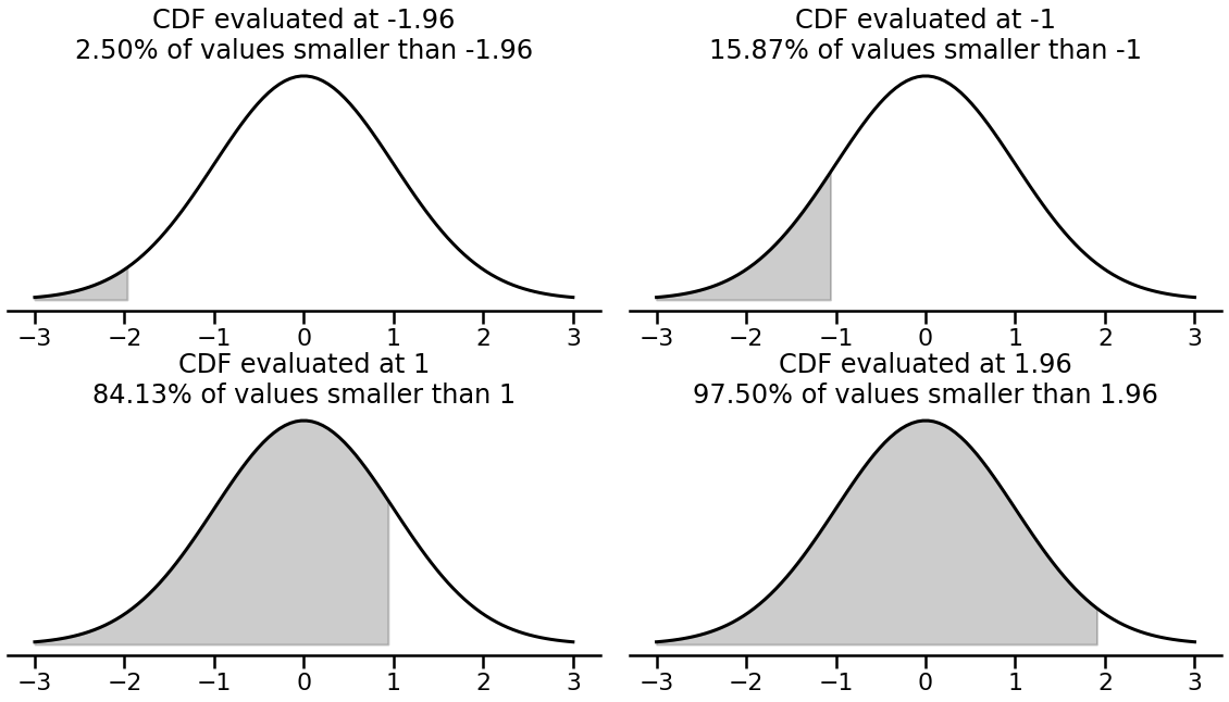
The shaded areas above represent the probability that a value from the distribution is less than the evaluated value. So for example, only 2.5% of samples are smaller than -1.96 in a standard normal. Its this property that allows probit regression to offer probabilities that allow for the classification of binary observations. Lets see how this is done below, which is traditionally simple at this point - we will refit the logistic regression model above using probit regression:
# Use probit
probit_results = smf.probit('idp ~ disea + mdvis + lncoins', data=rand).fit()

# Probit summary
probit_results.summary()
Optimization terminated successfully.
         Current function value: 0.538534
         Iterations 5
| Dep. Variable: | idp | No. Observations: | 20190 |
|---|---|---|---|
| Model: | Probit | Df Residuals: | 20186 |
| Method: | MLE | Df Model: | 3 |
| Date: | Sat, 09 Jul 2022 | Pseudo R-squ.: | 0.06021 |
| Time: | 11:56:15 | Log-Likelihood: | -10873. |
| converged: | True | LL-Null: | -11570. |
| Covariance Type: | nonrobust | LLR p-value: | 8.895e-302 |
| coef | std err | z | P>|z| | [0.025 | 0.975] | |
|---|---|---|---|---|---|---|
| Intercept | -0.3798 | 0.020 | -18.608 | 0.000 | -0.420 | -0.340 |
| disea | 0.0077 | 0.001 | 5.225 | 0.000 | 0.005 | 0.011 |
| mdvis | -0.0253 | 0.002 | -10.188 | 0.000 | -0.030 | -0.020 |
| lncoins | -0.1813 | 0.005 | -35.678 | 0.000 | -0.191 | -0.171 |
Contrasting that with the logistic_results object, things will look very similar in terms of significance and direction of effects. However, how we interpret the coefficents is different. We no longer think of changes in log-odds here, but the change in the value of the unobserved, latent variable that gave rise to our binary observations, in much the same way one interprets ordinary least squares regression. Whether this is easier is a matter of taste; but you can actually scale probit coefficients by about 1.6 to get the log-odds given by a logistic regression - try it with the parameters above for the probit and logistic regressions!
Finally, we can examine the predictions of the probit model using the .fittedvalues attribute as before:
# View first 5 fitted values
display(probit_results.fittedvalues.head(5))
0   -1.110182
1   -1.160742
2   -1.110182
3   -1.110182
4   -1.110182
dtype: float64
These are not probabilities - these are the predictions of the latent normal variable. To get the probabilities, we can either use the .predict method which will convert it for us, or, we can take these fitted values and put them into a standard normal cumulative density function to get the probability of values being smaller than the given value:
# Use norm.cdf
norm(0, 1).cdf(probit_results.fittedvalues)
array([0.13346028, 0.12287333, 0.13346028, ..., 0.1376718 , 0.1376718 ,
       0.14910515])
And there they are - those probabilities can now be interpreted as the probability an observed binary outcome is zero or one. Traditionally the cutoff is set at .50 like in logistic regression; but this is something a researcher needs to define in advance. Confusion matrices and so on can be computed in the usual way.
3.3. Ordered Probit Regression#
When you have binary data, logistic or probit regression are great tools to have, albeit with different philosophies. There is a particular class of problem, however, that the latent variable approach of probit regression has great clarity for. In psychology, many studies use Likert (“lick-ert”) scales to collect behavioural responses. Participants may rate how much they agree with a statement or have a preference for a particular stimulus on a scale from 1-7 or -3 to +3, or many other variants.
Traditionally, this data is analysed with ordinary least squares. But a moment’s reflection illustrates this could be misguided. Participants are forced to response on whole, ordered numbers, but the spacing between those numbers may not be consistent - there’s no way to say that a 3 and a 4 on a 7-point scale have the same intrinsic difference as a 6 and a 7. If you’re predicting values its also worth making sure the predictions resemble the data, which ordinary least squares won’t give you. Indeed, there is a lot of work from the last few years illustrating the issues with predicting ordinal data using ordinary least squares.
We will investigate the use of ordinal regression here, which is capable of solving the above problem. There are many ways to fit a model to ordinal data, but the one we’ll discuss here is a direct continuation of probit regression, sometimes called ordered probit regression. The extension is very natural. In probit regression with binary data, we used the cumulative density function of a normal distribution to get probabilities that a datapoint belongs to either class. In ordered probit regression, in addition to estimating the coefficients, we estimate a series of cutpoints that carve up the cumulative density function into sections. The model then predicts the latent variable, and we use the cumulative density function to get a probability. Then, we see which region of the distribution the probability falls into. Lets see an example.
with sns.plotting_context('poster'):

    # Make figure
    fig, (count, ax) = plt.subplots(1, 2, figsize=(20, 10))
    sns.despine(ax=ax, left=True)
    sns.despine(ax=count)
    ax.set(yticklabels=[], yticks=[])

    # Plot pdf
    ax.plot(x := np.linspace(-4, 4, 100), y := standard_normal.pdf(x), linestyle='-', color='black', linewidth=3)

    # Get a few cutpoints
    cutpoints = [-0.75, 0.1, 1.5]

    # Add scatter + shading
    ax.scatter(cutpoints, standard_normal.pdf(cutpoints), s=500, color='black')
    for c, alpha in zip(cutpoints, [.5, .4, .3]):
        ax.fill_between(x, y, where=(standard_normal.cdf(x) < standard_normal.cdf(c)),
                        color='black', alpha=alpha)

    # Get ordinal data
    ordinal = np.digitize(norm(0, 1).rvs(1000), bins=cutpoints) + 1

    # Plot ordinal
    sns.countplot(x=ordinal, ax=count, palette='Greys_r', edgecolor='black')
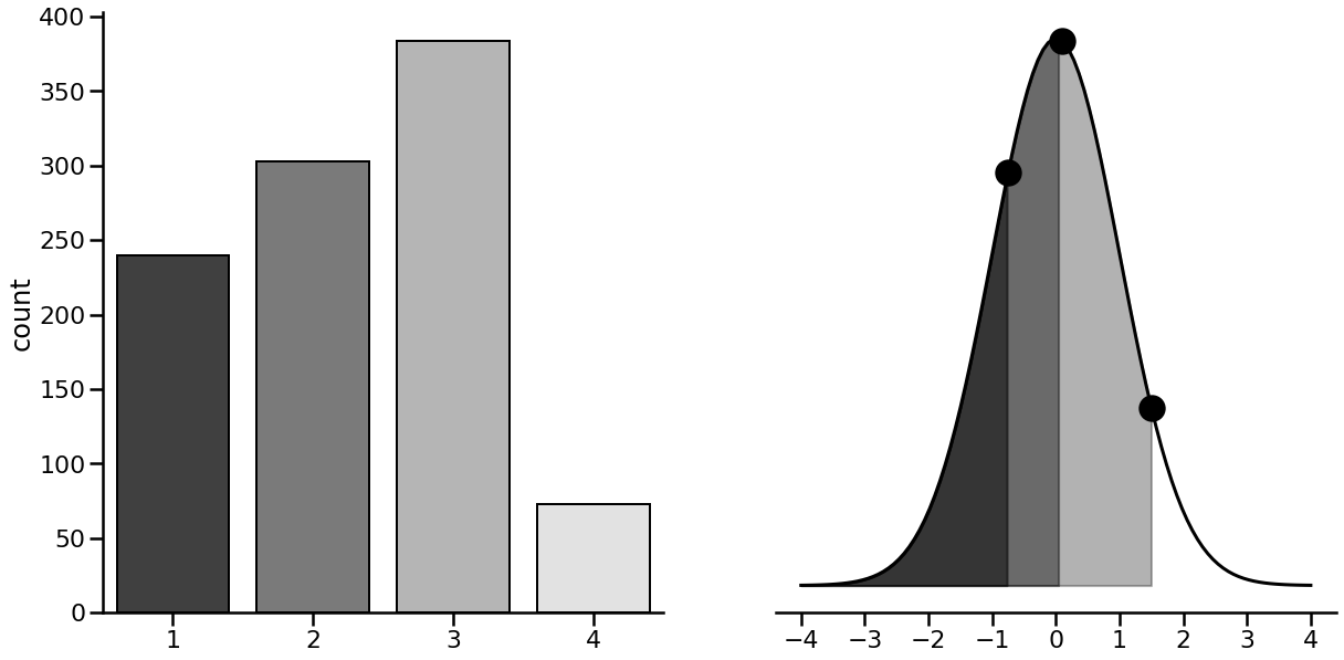
In this imaginary dataset, we have a 1,000 data points where responses have been recorded on a scale of 1-4. The figure on the left represents the counts of the observed responses - e.g., 3 is the most common, 4 the least, and so on. The right figure shows the standard normal distribution with three points along the curve, and shaded regions. The points represent the cutpoints, which highlight where a response changes from a 1 to a 2, and so on. The shaded regions represent the areas of the cumulative density function - the greater the shaded area, the more probable a response is. Its clear the lighter shaded region in the 0 - 1.5 area is tied with a greater probability of a response, and indeed ‘3’ is the most common response.
In this example, we know the cutpoints. As such, we can work out the probability regions via subtraction, and see which probability regions are associated with a response.
For the ‘1’ responses, the CDF up to a cutpoint of -0.75 will give the probability.
For the ‘2’ responses, the CDF up to -0.75 subtracted from the cutpoint at 0.1 will give the probability.
For the ‘3’ responses, the CDF up to 0.1 subtracted from the cutpoint at 1.5 will give the probability.
For the ‘4’ responses, 1 - the CDF up to 1.5 will give the final probability.
Let’s compute these using the standard_normal object.
# Known cuts
known_cutpoints = [-0.75, 0.1, 1.5]
cut1 = standard_normal.cdf(known_cutpoints[0])
cut2 = standard_normal.cdf(known_cutpoints[1]) - standard_normal.cdf(cutpoints[0])
cut3 = standard_normal.cdf(known_cutpoints[2]) - standard_normal.cdf(cutpoints[1])
cut4 = 1 - standard_normal.cdf(known_cutpoints[2])

pr = np.array([cut1, cut2, cut3, cut4]).round(2)

print(pr)
[0.23 0.31 0.39 0.07]
The probabilities map cleanly onto the actual observed data.
OK - that’s the latent variable model of ordinal, probit regression. How can we estimate this in Python, and how can we interpret it? We will fit an ordered probit model below, using the Affairs dataset, which contains data on marital satisfaction (rated on a 1-5 scale), with other variables such as age, years married, and number of children. There are a few more, but we will focus on the latter two.
# Load the dataset
affairs = sm.datasets.fair.load().data
affairs.head()
| rate_marriage | age | yrs_married | children | religious | educ | occupation | occupation_husb | affairs | |
|---|---|---|---|---|---|---|---|---|---|
| 0 | 3.0 | 32.0 | 9.0 | 3.0 | 3.0 | 17.0 | 2.0 | 5.0 | 0.111111 |
| 1 | 3.0 | 27.0 | 13.0 | 3.0 | 1.0 | 14.0 | 3.0 | 4.0 | 3.230769 |
| 2 | 4.0 | 22.0 | 2.5 | 0.0 | 1.0 | 16.0 | 3.0 | 5.0 | 1.400000 |
| 3 | 4.0 | 37.0 | 16.5 | 4.0 | 3.0 | 16.0 | 5.0 | 5.0 | 0.727273 |
| 4 | 5.0 | 27.0 | 9.0 | 1.0 | 1.0 | 14.0 | 3.0 | 4.0 | 4.666666 |
We will try to predict rate_marriage from yrs_married and number of children. But first, we need to set the rate_marriage variable as an ordered category, which we do with pandas pd.Categorical function:
# Convert to categorical
affairs['marriage_category'] = pd.Categorical(affairs['rate_marriage'], categories=[1, 2, 3, 4, 5], ordered=True)
affairs.head()
| rate_marriage | age | yrs_married | children | religious | educ | occupation | occupation_husb | affairs | marriage_category | |
|---|---|---|---|---|---|---|---|---|---|---|
| 0 | 3.0 | 32.0 | 9.0 | 3.0 | 3.0 | 17.0 | 2.0 | 5.0 | 0.111111 | 3 |
| 1 | 3.0 | 27.0 | 13.0 | 3.0 | 1.0 | 14.0 | 3.0 | 4.0 | 3.230769 | 3 |
| 2 | 4.0 | 22.0 | 2.5 | 0.0 | 1.0 | 16.0 | 3.0 | 5.0 | 1.400000 | 4 |
| 3 | 4.0 | 37.0 | 16.5 | 4.0 | 3.0 | 16.0 | 5.0 | 5.0 | 0.727273 | 4 |
| 4 | 5.0 | 27.0 | 9.0 | 1.0 | 1.0 | 14.0 | 3.0 | 4.0 | 4.666666 | 5 |
OK, this looks perfect. Fitting the model is somewhat more involved as ordinal regression isn’t under the usual statsmodels.formula.api. We import it from the miscmodels.ordinal_model namespace, like so:
# Import ordinal model
from statsmodels.miscmodels.ordinal_model import OrderedModel
We also can’t fit this directly with a formula as we have done above. Instead, we use the from_formula attribute and fit it as normal, specifying the distr keyword as ‘probit’.
# Fit the model
ordered_probit = OrderedModel.from_formula('marriage_category ~ yrs_married + children',
                                           data=affairs, distr='probit')

# Fit the model
ordered_results = ordered_probit.fit()

# Show summary
ordered_results.summary()
Optimization terminated successfully.
         Current function value: 1.236414
         Iterations: 267
         Function evaluations: 426
| Dep. Variable: | marriage_category | Log-Likelihood: | -7871.0 |
|---|---|---|---|
| Model: | OrderedModel | AIC: | 1.575e+04 |
| Method: | Maximum Likelihood | BIC: | 1.579e+04 |
| Date: | Sat, 09 Jul 2022 | ||
| Time: | 11:56:16 | ||
| No. Observations: | 6366 | ||
| Df Residuals: | 6360 | ||
| Df Model: | 6 |
| coef | std err | z | P>|z| | [0.025 | 0.975] | |
|---|---|---|---|---|---|---|
| yrs_married | -0.0103 | 0.003 | -3.470 | 0.001 | -0.016 | -0.004 |
| children | -0.0558 | 0.015 | -3.714 | 0.000 | -0.085 | -0.026 |
| 1/2 | -2.3552 | 0.045 | -52.493 | 0.000 | -2.443 | -2.267 |
| 2/3 | -0.3653 | 0.052 | -6.967 | 0.000 | -0.468 | -0.263 |
| 3/4 | -0.3110 | 0.029 | -10.625 | 0.000 | -0.368 | -0.254 |
| 4/5 | -0.0420 | 0.018 | -2.304 | 0.021 | -0.078 | -0.006 |
We get two coefficients for the predictors, but notice here we also get interesting extra rows - 1/2, 2/3, 3/4, 4/5. These represent the cutpoints - where responses switch from one to another. The coefficients are interpreted in much the same way as probit regression - one unit increases in the predictor are associated with a coefficient-value change in the latent variable. Somewhat frustratingly, the cutpoints are given on a different scale to the underlying latent variable. Fortunately, we can convert them using the models .transform_threshold_params. Let’s take a look:
# Transform the cutpoints
n_cuts = 4
ordered_probit.transform_threshold_params(ordered_results.params[-n_cuts:])
array([       -inf, -2.35518476, -1.661222  , -0.92852619,  0.03032953,
               inf])
Those cutpoints show where along the distribution the switchpoints are. How to recover the predictions of an ordinal model? There is no .fittedvalues attribute here, but if we examine the .predict() output of the model, we will see something interesting:
# Use the model to predict
ordered_results.predict()
array([[0.01806795, 0.06247448, 0.17128938, 0.3623057 , 0.3858625 ],
       [0.01997206, 0.06688539, 0.17825335, 0.36463794, 0.37025126],
       [0.00991585, 0.04105062, 0.13233409, 0.33902752, 0.47767191],
       ...,
       [0.00991585, 0.04105062, 0.13233409, 0.33902752, 0.47767191],
       [0.01261749, 0.04869801, 0.14733056, 0.35007508, 0.44127886],
       [0.00991585, 0.04105062, 0.13233409, 0.33902752, 0.47767191]])
This array represents the probability that each observation (the rows) belongs to each bin along the sliced up distribution (each column). For example, the first column would be the probability the response to marital satisfaction is ‘1’. To recover actual points, we simply take the maximum, which is perhaps clearer in a pandas dataframe:
# Set up ordinal predictions
ordinal_predictions = pd.DataFrame(ordered_results.predict(),
                                   columns=affairs['marriage_category'].cat.categories)

# Show the predictions
ordinal_predictions.idxmax(axis='columns')
0       5
1       5
2       5
3       4
4       5
       ..
6361    5
6362    5
6363    5
6364    5
6365    5
Length: 6366, dtype: int64
These can then be compared with the observed data using confusion-matrix based approaches.
3.4. Poisson or Negative Binomial models#
Though not encountered too often in psychological science, data that are distributed as counts are popular across other fields and are becoming more popular in behavioural research. Count data represent data that are coded as whole numbers (integers) that start at zero and have no upper limit. Normal regression models like ordinary least squares may make negative count predictions, or fractional predictions, which make little sense (what does it mean to have, say, negative counts of a behaviour?).
Fortunately, count data can be modelled relatively simply with either a \(Poisson\) or \(Negative Binomial\) regression. These models are named after the distributions of the same name which describe the probability of count data. The Poisson is a straightforward single-parameter distribution that describes distributions of counts. The single parameter is sometimes called the ‘rate’, and it represents the average of all the count data in a Poisson distribution. So while the Poisson distribution produces whole-integer values, its parameter can be a continuous (positive!) value.
The negative binomial is traditionally used to describe the probability of observing a number of failures before a single success - e.g. how many times must I roll a dice before I get a 3? The number of ‘fails’ (roll != 3) would be modelled by the negative binomial.
Sometimes, the single-parameter Poisson does a good enough job in regression contexts. However sometimes we encounter a phenomenon called over-dispersion, which is where the variability of the counts exceeds the average tendency. Fortunately, the negative binomial can be used instead, as it allows for a second parameter to incorporate the variability.
If this sounds too technical, don’t worry - it really is. The details are not vital; what we need to focus on is if we are dealing with count data, we can start with the Poisson model, check for this overdispersion, and if it appears, switch to the negative binomial.
3.4.1. Poisson Regression#
Using the rand data, we could think of a different research question, asking whether the number of medical visits mdvis (a count variable!) is influenced by the coinsurance payment lncoins, as well as the number of chronic diseases, disea. Doing this in statsmodels is very easy - same idea as before; get the formula ready and use the Poisson function!
# Fit a Poisson regression
poisson_results = smf.poisson('mdvis ~ lncoins + disea', data=rand).fit()

# Summarise
poisson_results.summary()
Optimization terminated successfully.
         Current function value: 3.141408
         Iterations 5
| Dep. Variable: | mdvis | No. Observations: | 20190 |
|---|---|---|---|
| Model: | Poisson | Df Residuals: | 20187 |
| Method: | MLE | Df Model: | 2 |
| Date: | Sat, 09 Jul 2022 | Pseudo R-squ.: | 0.04835 |
| Time: | 11:56:16 | Log-Likelihood: | -63425. |
| converged: | True | LL-Null: | -66647. |
| Covariance Type: | nonrobust | LLR p-value: | 0.000 |
| coef | std err | z | P>|z| | [0.025 | 0.975] | |
|---|---|---|---|---|---|---|
| Intercept | 0.6474 | 0.009 | 75.120 | 0.000 | 0.630 | 0.664 |
| lncoins | -0.0597 | 0.002 | -27.788 | 0.000 | -0.064 | -0.055 |
| disea | 0.0409 | 0.001 | 81.383 | 0.000 | 0.040 | 0.042 |
Great, some results! What do these mean again?
Like logistic regression, Poisson regression uses a special kind of function to transform the outcome variable in order to model it. It uses a log-transform, which means the coefficients are on the log-scale. That is, as the predictor increases, the log-count of the variable increases by one. As before we can exponentiate these:
# Exponentiate
display(np.exp(poisson_results.params))
Intercept    1.910517
lncoins      0.942055
disea        1.041777
dtype: float64
That is somewhat clearer - as the number of diseases increases, so does the count of doctors visits. And, as the premium goes up, the number of visits go down. This makes sense, the pricier it is to get healthcare, the less likely you are to go.
As with other kinds of generalized linear models, its often easier to work with the predictions directly to draw some conclusions. If we call the .predict method on fitted Poisson regression model, we will get the predictions back with no transformations needed. If you want to verify its correct you can exponentiate the .fittedvalues attribute and you will get the same results!
# Call predict and store the predictions in the rand dataframe
rand['predicted_mdvis'] = poisson_results.predict()

display(rand.head())
| mdvis | lncoins | idp | lpi | fmde | physlm | disea | hlthg | hlthf | hlthp | predictions | predicted_idp | predicted_mdvis | |
|---|---|---|---|---|---|---|---|---|---|---|---|---|---|
| 0 | 0 | 4.61512 | 1 | 6.907755 | 0.0 | 0.0 | 13.73189 | 1 | 0 | 0 | 0.129403 | 0 | 2.544425 |
| 1 | 2 | 4.61512 | 1 | 6.907755 | 0.0 | 0.0 | 13.73189 | 1 | 0 | 0 | 0.118646 | 0 | 2.544425 |
| 2 | 0 | 4.61512 | 1 | 6.907755 | 0.0 | 0.0 | 13.73189 | 1 | 0 | 0 | 0.129403 | 0 | 2.544425 |
| 3 | 0 | 4.61512 | 1 | 6.907755 | 0.0 | 0.0 | 13.73189 | 1 | 0 | 0 | 0.129403 | 0 | 2.544425 |
| 4 | 0 | 4.61512 | 1 | 6.907755 | 0.0 | 0.0 | 13.73189 | 1 | 0 | 0 | 0.129403 | 0 | 2.544425 |
Something unusual is going on. The predicted values are floating numbers, not count data. Whats happening here? Much like with ordinary least squares and logistic regression, Poisson regression is predicting the expected value of the observed data point - essentially, what the average value of that data point would be, given its values on the predictors. So what we are really looking at here is the parameter or ‘rate’ of the distribution that the data point came from!
We can expand our fishing adventures by using an alternative function in the results object of a Poisson regression, .predict_prob. This function takes the predicted rate (our predicted_mdvis variable above, and it does something quite clever:
It takes all the whole numbers from zero the maximum count value observed in the data.
For each datapoint, it takes the predicted rate, and builds a probability mass function from a Poisson distribution with that rate. What’s a probability mass function?! Its just the probability of seeing a specific count value, given a particular Poisson ‘rate’.
It returns all of those probabilities to us, and we can see what has the highest value - the most probable count value of our data.
This is going to be a little tricky to unpack, so lets do this step by step in the order above.
# Build a set of values from zero to the maximum observed in our data
# We add one because of Pythons 'up to but don't include' rule - see chapter 1!
counts = np.arange(0, max(rand['mdvis'] + 1))

# Get the probability mass of each datapoint, given the predicted rate!
probability_mass = poisson_results.predict_prob()

# Put these in a dataframe
prob_mass_df = pd.DataFrame(probability_mass, columns=counts)
display(prob_mass_df.head(2))
| 0 | 1 | 2 | 3 | 4 | 5 | 6 | 7 | 8 | 9 | ... | 68 | 69 | 70 | 71 | 72 | 73 | 74 | 75 | 76 | 77 | |
|---|---|---|---|---|---|---|---|---|---|---|---|---|---|---|---|---|---|---|---|---|---|
| 0 | 0.078518 | 0.199784 | 0.254167 | 0.21557 | 0.137125 | 0.069781 | 0.029592 | 0.010756 | 0.003421 | 0.000967 | ... | 1.203950e-70 | 4.439651e-72 | 1.613766e-73 | 5.783247e-75 | 2.043755e-76 | 7.123537e-78 | 2.449365e-79 | 8.309635e-81 | 2.782006e-82 | 9.192993e-84 |
| 1 | 0.078518 | 0.199784 | 0.254167 | 0.21557 | 0.137125 | 0.069781 | 0.029592 | 0.010756 | 0.003421 | 0.000967 | ... | 1.203950e-70 | 4.439651e-72 | 1.613766e-73 | 5.783247e-75 | 2.043755e-76 | 7.123537e-78 | 2.449365e-79 | 8.309635e-81 | 2.782006e-82 | 9.192993e-84 |
2 rows × 78 columns
OK! Only two datapoints are shown but we have the probability that the datapoint is the count shown in the DataFrame header, given the predicted rate. If we want to collapse this into a single number, all we need to is take index with the maximum value (i.e. , for row one, what is the column with the highest probability?)
pandas can help here, with the .idxmax method.
# Assign this back to the rand data
rand['predicted_count_mdvis'] = prob_mass_df.idxmax(axis='columns')

display(rand.head())
| mdvis | lncoins | idp | lpi | fmde | physlm | disea | hlthg | hlthf | hlthp | predictions | predicted_idp | predicted_mdvis | predicted_count_mdvis | |
|---|---|---|---|---|---|---|---|---|---|---|---|---|---|---|
| 0 | 0 | 4.61512 | 1 | 6.907755 | 0.0 | 0.0 | 13.73189 | 1 | 0 | 0 | 0.129403 | 0 | 2.544425 | 2 |
| 1 | 2 | 4.61512 | 1 | 6.907755 | 0.0 | 0.0 | 13.73189 | 1 | 0 | 0 | 0.118646 | 0 | 2.544425 | 2 |
| 2 | 0 | 4.61512 | 1 | 6.907755 | 0.0 | 0.0 | 13.73189 | 1 | 0 | 0 | 0.129403 | 0 | 2.544425 | 2 |
| 3 | 0 | 4.61512 | 1 | 6.907755 | 0.0 | 0.0 | 13.73189 | 1 | 0 | 0 | 0.129403 | 0 | 2.544425 | 2 |
| 4 | 0 | 4.61512 | 1 | 6.907755 | 0.0 | 0.0 | 13.73189 | 1 | 0 | 0 | 0.129403 | 0 | 2.544425 | 2 |
OK, now we have predicted counts! What does that look like?
sns.scatterplot(y=rand['mdvis'], x=rand['predicted_count_mdvis'])
<AxesSubplot:xlabel='predicted_count_mdvis', ylabel='mdvis'>
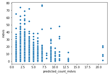
Not great, sadly. The model is really under-predicting - the observed data goes from 0 to 77, but the predictions only top 20. Is our data over-dispersed? We can check this, but it involves a little manual calculation - nothing too bad, though. First we take the models Pearson residuals, square them, and sum them. Then we divide this by the residual degrees of freedom of the model. If the result is greater than 1, we have evidence of overdispersion and should switch our modelling strategy.
# Compute overdispersion
od = (poisson_results.resid_pearson ** 2 ).sum() / poisson_results.df_resid

print(od, od > 1)
6.437470502281646 True
That might explain our not-so-good predictions.
3.4.2. Negative Binomial Regression#
Fitting a negative binomial regression at this point should be intuitive - we simply set up the formula, and pass it directly to the negativebinomial function:
# Fit the model
negbinom_results = smf.negativebinomial('mdvis ~ lncoins + disea', data=rand).fit()

# Get summary
negbinom_results.summary()
Optimization terminated successfully.
         Current function value: 2.159078
         Iterations: 13
         Function evaluations: 16
         Gradient evaluations: 16
| Dep. Variable: | mdvis | No. Observations: | 20190 |
|---|---|---|---|
| Model: | NegativeBinomial | Df Residuals: | 20187 |
| Method: | MLE | Df Model: | 2 |
| Date: | Sat, 09 Jul 2022 | Pseudo R-squ.: | 0.01374 |
| Time: | 11:56:17 | Log-Likelihood: | -43592. |
| converged: | True | LL-Null: | -44199. |
| Covariance Type: | nonrobust | LLR p-value: | 1.480e-264 |
| coef | std err | z | P>|z| | [0.025 | 0.975] | |
|---|---|---|---|---|---|---|
| Intercept | 0.6264 | 0.020 | 31.766 | 0.000 | 0.588 | 0.665 |
| lncoins | -0.0633 | 0.005 | -13.482 | 0.000 | -0.072 | -0.054 |
| disea | 0.0431 | 0.001 | 31.612 | 0.000 | 0.040 | 0.046 |
| alpha | 1.3365 | 0.019 | 70.288 | 0.000 | 1.299 | 1.374 |
The interpretation of the coefficients is much the same as the Poisson regression case, with the estimates representing the change in the log-counts of the outcome variable with a one-unit change in the predictor variable. Exponentiating them casts them on an odds scale.
You may notice the model seems to have an extra estimate - alpha - that also has a significance test associated with it. This is the overdispersion parameter. Recall that the Poisson distribution has a single parameter, the ‘rate’, or average. If the counts vary a lot, the Poisson will find it difficult to model the variability with a single parameter. The negative binomial distribution has a similar rate or average, but also has an additional parameter, alpha, which controls the variability of the counts. The model tests whether this value is significantly different from zero, which seems to be the case here. It’s another way of examining over-dispersion! Interestingly, if this parameter equals zero, the model is mathematically equivalent to a Poisson regression.