3. Advanced plotting with seaborn

How can you plot even more variables in a dataset? Sometimes, your experimental design will move beyond two categorical predictors into three or more. How can those be visualised? seaborn provides a few figure-level plotting options, which essentially means it will create the specified number of axes and subplots as is required. For example, in the exercise dataset, there is another variable we haven’t looked at - time.

Something called catplot allows us to examine this, short for category plot.

# Catplot example
cat = sns.catplot(data=exercise, x='kind', y='pulse', 
                  hue='diet', col='time', kind='violin', split=True)

catplot allows you to spread different variables onto columns or rows, as well as specify the kind of plot using the kind keyword.

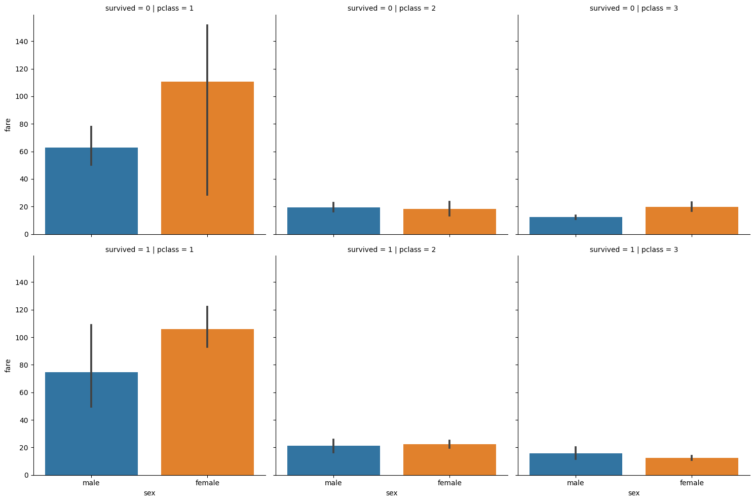
# Titanic data, examining cost of tickets for men/women
# PER class and survival
titanic = sns.load_dataset('titanic')

cat2 = sns.catplot(data=titanic, y='fare', x='sex', 
                   row='survived', col='pclass', kind='bar')

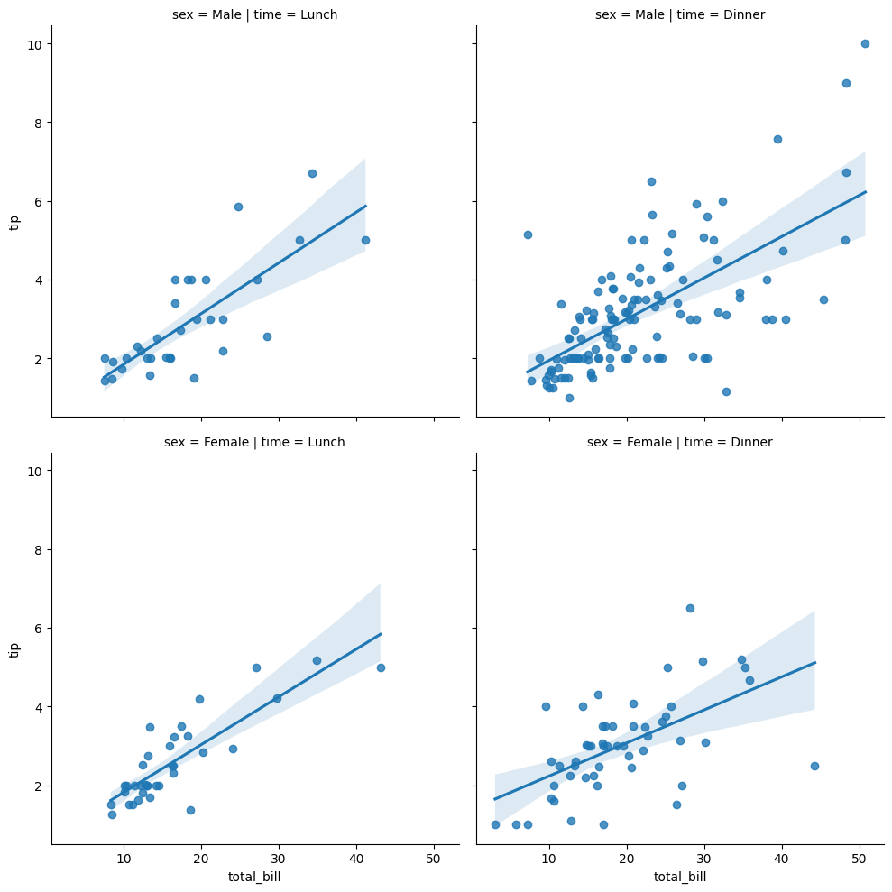
In a similar vein, lmplot is capable of visualising relationships between continuous variables. Essentially, this is a scatter plot, but also fits a regression line for you.

# Show lmplot on tips data
sns.lmplot(data=tips, x='total_bill', y='tip', col='time', row='sex')

<seaborn.axisgrid.FacetGrid at 0x13424e3b0>

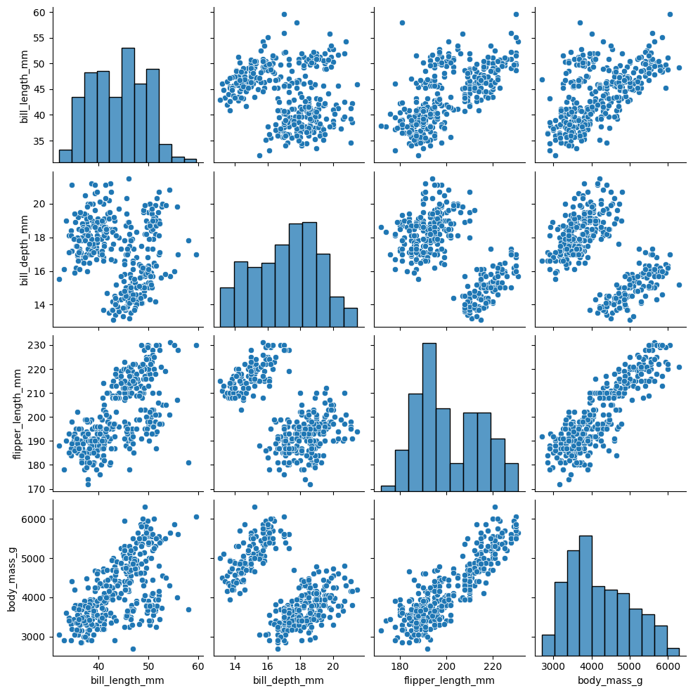
There is also pairplot, which highlights bivariate and univariate relationships for all continuous variables in a dataset. We can examine this in the penguins dataset, which describes various body measurements for different species of penguins:

# load penguins
penguins = sns.load_dataset('penguins')

# Simple but powerful
sns.pairplot(penguins)

<seaborn.axisgrid.PairGrid at 0x131d41420>

Finally, seaborn has a special class of plot that helps with splitting datasets up by certain variables, called FacetGrid. Interestingly, FacetGrid does not plot anything on its own - it simply lays out a grid of plots specific to the variable you want. It has a .map_dataframe method that allows you to send specific plotting commands to the sub-groups of your data. It’s somewhat tricky but extremely flexible. Below, we split the up the diamonds dataset, which contains a range of information on diamond cut, quality, price, and other measures.

# Load diamonds
diamonds = sns.load_dataset('diamonds')

display(diamonds.head())

	carat	cut	color	clarity	depth	table	price	x	y	z
0	0.23	Ideal	E	SI2	61.5	55.0	326	3.95	3.98	2.43
1	0.21	Premium	E	SI1	59.8	61.0	326	3.89	3.84	2.31
2	0.23	Good	E	VS1	56.9	65.0	327	4.05	4.07	2.31
3	0.29	Premium	I	VS2	62.4	58.0	334	4.20	4.23	2.63
4	0.31	Good	J	SI2	63.3	58.0	335	4.34	4.35	2.75

Lets attempt to plot the relationship between price and carat for each level of cut and color, and add colours to each datapoint depending on their clarity. Phew! The below cell is hidden but shows how seaborn cleverly divides a plot up into the respective subplots with no additional work from us:

# The initial call to FacetGrid takes the dataset and what you want to put in the rows and columns:
sns.FacetGrid(data=diamonds, row='cut', col='color')

<seaborn.axisgrid.FacetGrid at 0x1349d8c10>

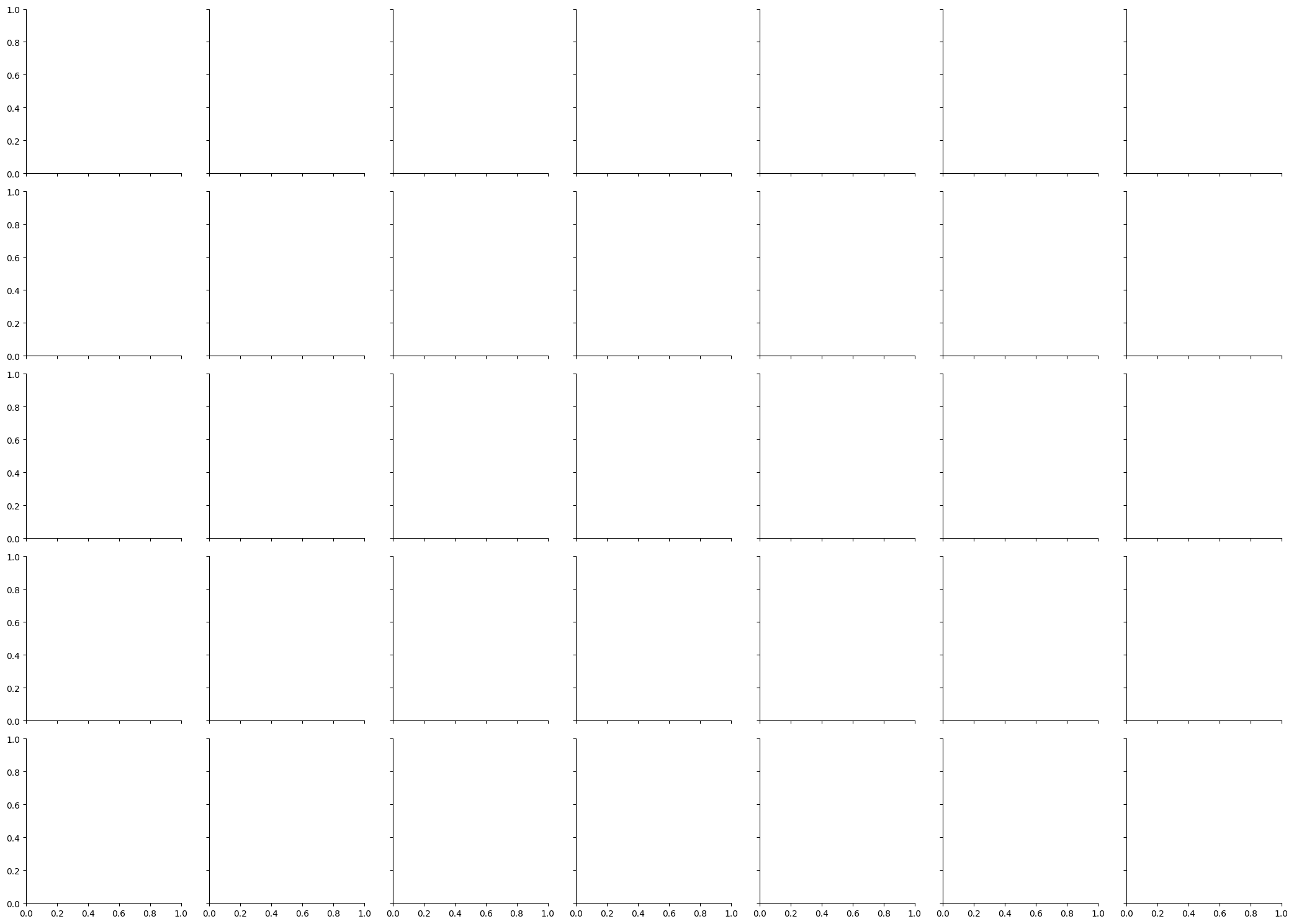
As can be seen, a blank canvas is created that pairs every unique combination of cut and color. We now add what we want using the .map_dataframe method, sending in the sns.scatterplot function, with our x, y, and hue variables:

# Map dataframe (as in, map the plotting function to the group-dataframes0
(
    sns.FacetGrid(data=diamonds, row='cut', col='color')
    .map_dataframe(sns.scatterplot, x='carat',
                   y='price', hue='clarity')
    .add_legend() # need to add this to see the legend
)

<seaborn.axisgrid.FacetGrid at 0x135643610>

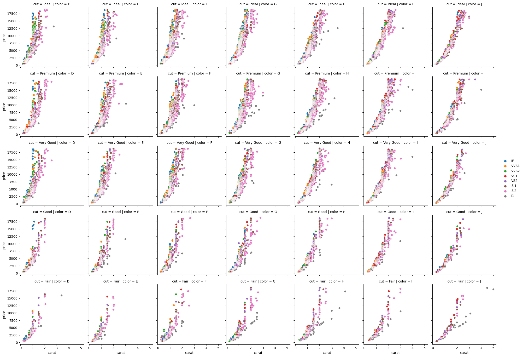
An amazing amount of data plotted in just a few lines. We could even add another .map_dataframe to add a different type of plot on top of the scatter. Custom plotting functions can also be defined and passed to .map_dataframe for highly customised plots.

3.1. Visualisation

You should be able to get data into any shape required for analysis, as well as producing a variety of clear and concise plots that show the relationships amongst the data. For the most part, seaborn requires DataFrames in the long format, so if your plot doesn’t look quite right, try to reformat your data through melting and pivoting.